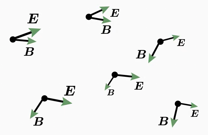
Electroencephalography (EEG) measures electric potentials on the scalp and magnetoencephalography (MEG) measures magnetic fields outside the head; both are generated by the same electric currents in the brain. This tutorial summarizes the electromagnetism needed to understand these signals, the equipment used to record them and the models used to analyze them. The last chapter, Electromagnetism of EEG and MEG, applies it to brain signals.
Charges (stationary or moving) and changing magnetic fields. Monopoles exist (positive and negative charges).
Moving charges (currents), intrinsic magnetic moments and changing electric fields. No magnetic monopoles have been observed.
Field Lines
Originate on positive charges, terminate on negative charges (or extend to infinity) when produced by charges.
Closed loops. No starting or ending points.
Units
V/m (volts per meter) or N/C
T (tesla) or V·s/m² (volt-seconds per square meter).
Force on a Charge
\(F = qE\) (electric component of the Lorentz force).
\(F = q(v \times B)\) (magnetic component of the Lorentz force).
Field Equations
Gauss’s Law: \(\nabla \cdot E = \frac{\rho}{\epsilon_0}\)
Gauss’s Law for Magnetism: \(\nabla \cdot B = 0\) (no magnetic monopoles).
Induction
Induced by changing magnetic fields (Faraday’s Law): \(\nabla \times E = -\partial B/\partial t\).
Induced by changing electric fields and by currents (Ampère-Maxwell Law).
Energy Storage
Energy density: \(\frac{1}{2}\epsilon_0 E^2\)
Energy density: \(\frac{1}{2\mu_0} B^2\)
Electric Charge
Nature of Charge
Positive Charge: More protons than electrons (e.g., a proton or a positively ionized atom).
Negative Charge: More electrons than protons (e.g., an electron or a negatively ionized atom).
Elementary Charge: The smallest unit of free charge, denoted \(e \approx 1.602 \times 10^{-19}\,\mathrm{C}\).
Electron charge: \(-e\)
Proton charge: \(+e\)
Coulomb (C): The charge carried by about \(6.24 \times 10^{18}\) elementary charges.
Quantization and Conservation
Quantization: Free charge is always an integer multiple of \(e\) (quarks carry \(\pm e/3\) and \(\pm 2e/3\) but are never observed free).
Conservation: In a closed system, the total charge remains constant. Charge can be redistributed but never created or destroyed.
Electric Field and Charge Distribution
Field Lines
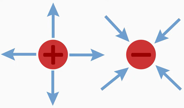
Positive Charge: Field lines radiate outward.
Negative Charge: Field lines radiate inward.
Conductors vs. Insulators
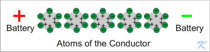
Conductors: Free electrons move easily. In electrostatic equilibrium, excess charge resides on the outer surface (mutual repulsion pushes it as far apart as possible), and the electric field inside is zero.
Insulators: Electrons are bound to atoms. Excess charge stays where it was placed (it does not redistribute).
Mathematical Descriptions
Separation Vector
Source Point (\(\mathbf{r}^\prime\)): Location of the charge.
Field Point (\(\mathbf{r}\)): Point where the field is calculated.
Separation Vector: \(\mathbf{R} = \mathbf{r} - \mathbf{r}^\prime\), with unit vector \(\hat{\mathbf{R}} = \mathbf{R}/\vert\mathbf{R}\vert\).
where: \(\epsilon_0\) is the permittivity of free space (\(8.85\times 10^{-12}\) F/m), \(\hat{\mathbf{r}}\) is the unit vector pointing from the charge to the field point.
Charge by Induction
Process:
Bring a negatively charged object near (without touching) a neutral conductor.
Electrons in the conductor are repelled to the far side; the near side becomes positively charged.
Ground the conductor so that electrons can leave.
Remove the grounding connection before removing the charged object.
Result: The conductor retains a net positive charge.
Energy and Voltage
Energy: \(W = qV\), where \(V\) is the voltage (potential difference) and \(q\) is the charge.
Voltage: The work done per unit charge to move charge between two points.
Practical Implications
Electrostatics: Used in photocopiers, air purifiers (electrostatic precipitators) and paint spraying.
Circuits: Charge flow (current) is fundamental to electronics and power systems.
Lightning: A dramatic example of charge separation and redistribution.
Electric Dipole
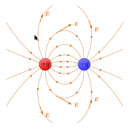
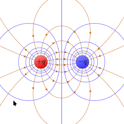
An electric dipole consists of two equal and opposite charges, \(+q\) and \(-q\), separated by a distance \(d\). Dipoles are fundamental to understanding electric fields, molecular behavior (e.g., polar water molecules) and antennas.
Dipole Moment (\(\vec{p}\))
The magnitude of the dipole moment is:
\[
\vert \vec{p} \vert = qd
\]
where: \(\vec{p}\) is the dipole moment vector, directed from the negative charge (\(-q\)) to the positive charge (\(+q\)), \(q\) is the magnitude of each charge (C), \(d\) is the distance between the charges (m).
Electric Field of a Dipole
The field at any point follows from the superposition principle. For distances much larger than the separation (\(r \gg d\)), where \(r\) is measured from the center of the dipole:
The dipole field falls off as \(1/r^3\), faster than the \(1/r^2\) of a point charge: at twice the distance, the field of a point charge decreases 4 times, that of a dipole 8 times. Because the brain sources of EEG and MEG are dipoles, their signals decrease steeply with the distance from the sensors, and deep sources contribute much less than superficial ones.
where: \(F_e\) is the electric force (N) between the two charges, \(Q\) and \(q\) are the charges (C); the sign of the product gives the direction (positive: repulsion, negative: attraction), \(r\) is the distance between the charges (m), \(\varepsilon_0\) is the permittivity of free space (\(8.85\times 10^{-12}\) F/m).
Interpretation
Magnitude: Proportional to the product of the charges and inversely proportional to the square of the distance.
Direction (along the line joining the charges):
Like charges (both positive or both negative) repel.
Opposite chargesattract.
Electric Force in an Electric Field
The force on a charge \(q\) placed in an electric field \(E\) is:
\[
F_e = qE
\]
where \(E\) is in N/C (equivalently V/m). The force is proportional to both the charge and the field strength.
Key Points
Superposition Principle: For multiple charges, the net force on a charge is the vector sum of the forces due to each individual charge.
Permittivity: In a material, \(\varepsilon_0\) is replaced by \(\varepsilon = \varepsilon_r \varepsilon_0\), where \(\varepsilon_r\) is the relative permittivity of the material.
Electric Field
Definition
The electric field\(E\) at a point is the electric force per unit charge on a (small, positive) test charge placed at that point:
\[
E = \frac{F_e}{q}
\]
where: \(E\) is the electric field (N/C or V/m), \(F_e\) is the electric force (N), \(q\) is the test charge (C).
Electric Field of a Point Charge
\[
E = \frac{1}{4 \pi \varepsilon_0} \frac{Q}{r^2}
\]
where \(Q\) is the source charge (C) and \(r\) is the distance from it (m).
The Coulomb constant\(k_e\) is related to \(\varepsilon_0\) by:
where: \(\hat{r}_i\) is the unit vector pointing from the \(i\)-th charge to the observation point, \(r_i\) is the distance from the \(i\)-th charge to the observation point.
The electric potential\(V\) due to a point charge \(q\) (zero at infinity) is:
\[
V = k_e \frac{q}{r}
\]
For multiple charges:
\[
V = k_e \sum_i \frac{q_i}{r_i}
\]
The field is the negative gradient of the potential:
\[
\vec{E} = -\nabla V
\]
For a uniform field (e.g., between parallel plates), the magnitude is:
\[
E = \frac{V}{d}
\]
where \(V\) is the potential difference (V) and \(d\) is the distance between the plates (m).
Electric Field Lines
Electric field lines are curves whose tangent at every point gives the direction of \(\vec{E}\) there. They can be constructed by placing a test charge at many points around the source charge \(Q\) and drawing the direction of the force on it.
Properties:
Tangency: The line direction at any point is the direction of \(\vec{E}\) at that point.
Density: The density of lines (number per unit area) is proportional to the magnitude of \(\vec{E}\). Denser lines mean a stronger field.
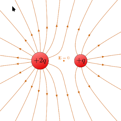
Origin and termination: Lines start on positive charges (or at infinity) and end on negative charges (or at infinity).
No crossing: Field lines never cross. A crossing would imply two different field directions at one point, which is impossible.
Field Line Patterns
A single positive charge: lines radiate outward in all directions.
A single negative charge: lines point inward from all directions.
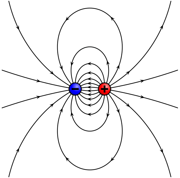
A dipole: lines start at the positive charge and end at the negative charge.
Electric Current
Definition
Electric current (\(I\)) is the rate of flow of electric charge through a cross-section of a conductor. It is measured in amperes (A):
\[
1 \, \text{A} = 1 \, \text{C/s}
\]
Mathematical Representation
\[
I = \frac{\mathrm{d}Q}{\mathrm{d}t}
\]
For a constant current:
\[
I = \frac{\Delta Q}{\Delta t}
\]
where \(\Delta Q\) is the total charge passing through the cross-section during the time interval \(\Delta t\).
The total charge transferred is the integral of the current:
\[
Q = \int I \, \mathrm{d}t
\]
Direction of Current Flow
Conventional current: Defined as the flow of positive charge, from the positive (+) to the negative (−) terminal of the source through the external circuit. The convention predates the discovery of the electron.
Electron flow: Electrons (negative) actually move from the negative to the positive terminal.
Key Point: The conventional current direction is opposite to the electron flow, but the effects (energy transfer, magnetic fields) are the same.
Current Density
The current density\(J\) is the current per unit cross-sectional area; it is treated in detail in its own chapter below. For a uniform current:
\[
J = \frac{I}{A}
\]
Practical Implications
Circuits: Current powers everything from household appliances to industrial machinery.
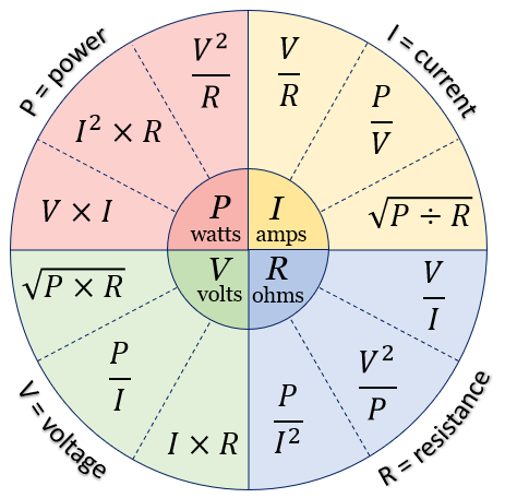
Ohm’s Law: \(I = V/R\) relates current, voltage and resistance.
Energy transfer: Current transfers electrical energy, enabling work to be done (lighting a bulb, running a motor).
Voltage
Definition
Voltage (electric potential difference) is the work done per unit charge in moving a charge between two points. It is measured in volts (V):
\[
1\,\text{V} = 1 \, \text{J/C}
\]
Mathematical Representation
\[
V = \frac{W}{q}
\]
where \(W\) is the work or energy (J) and \(q\) is the charge (C).
The potential difference between two points is:
\[
\Delta V = V_b - V_a
\]
Relationship with Electric Field
For a uniform electric field \(E\), the potential difference over a distance \(l\) along the field is:
\[
V = El
\]
where \(E\) is in V/m (or N/C) and \(l\) in m.
Electromotive Force (EMF)
EMF is the energy supplied per unit charge by a source (e.g., a battery). It is also measured in volts.
The terminal voltage is the voltage available to the circuit: EMF minus the drop across the source’s internal resistance.
Power
Power (\(P\)) is the rate at which energy is supplied or consumed, measured in watts (W):
\[
P = \frac{\mathrm{d}U}{\mathrm{d}t}
\]
where \(\mathrm{d}U\) is the change in energy (J) and \(\mathrm{d}t\) the time interval (s). For electrical power:
\[
P = VI
\]
Potential and Potential Difference
Electric potential at a point is the work per unit charge needed to bring a positive test charge from infinity to that point.
Potential difference (voltage) is the difference in potential between two points.
Resistance
Electrical Conductance (G)
Definition: How easily charge flows through a component.
Unit: siemens (S)
Relationship: \(G = \frac{1}{R}\)
Electrical Resistance (R)
Definition: How strongly a component opposes the flow of charge.
Unit: ohm (\(\Omega\))
Relationship: \(R = \frac{V}{I}\)
For a uniform conductor: \(R = \frac{\rho l}{A}\), where:
\(\rho\) is the resistivity of the material (\(\Omega \cdot \text{m}\)),
\(l\) is the length of the conductor (m),
\(A\) is the cross-sectional area (m²).
Resistivity (\(\rho\))
Definition: A material property quantifying how strongly it resists current.
Unit: ohm-meter (\(\Omega \cdot \text{m}\))
Relationship: \(\rho = \frac{E}{J}\), where \(E\) is the electric field (V/m) and \(J\) the current density (A/m²).
Conductivity (\(\sigma\))
Definition: The inverse of resistivity; how well a material conducts current.
Unit: siemens per meter (S/m)
Relationship: \(\sigma = \frac{1}{\rho}\)
Ohm’s Law
Basic Form
The current\(I\) through a conductor is proportional to the voltage\(V\) across it and inversely proportional to its resistance\(R\):
\[
V = IR
\]
where \(V\) is in volts, \(I\) in amperes and \(R\) in ohms. Ohm’s law holds for ohmic materials, for which \(R\) is constant (independent of \(V\)).
Vector Form
In electromagnetism and materials science, Ohm’s law is expressed with the current density\(J\) and the electric field\(E\):
\[
\vec{J} = \sigma \vec{E}
\]
where \(J\) is in A/m², \(\sigma\) in S/m and \(E\) in V/m. This form is useful for materials with varying conductivity and for three-dimensional current flow.
Impedance
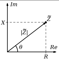
Impedance (\(Z\)) generalizes resistance to alternating current (AC) circuits. It accounts for both resistance and reactance (from capacitors and inductors) and is a complex number:
\[
Z = R + jX
\]
where: \(R\) is the resistance (\(\Omega\)), \(X\) is the reactance (\(\Omega\)), \(j\) is the imaginary unit (\(j^2 = -1\)).
Reactance is the opposition of a capacitor or inductor to alternating current. Unlike resistance, it depends on frequency and does not dissipate energy as heat. It is measured in ohms:
where \(\omega = 2\pi f\), \(C\) is the capacitance (F) and \(L\) the inductance (H). The reactance of a capacitor decreases with frequency (a capacitor blocks DC and passes high frequencies), that of an inductor increases with frequency.
Electrode impedance: the contact between an EEG electrode and the skin behaves like a resistor in parallel with a capacitor, so its impedance depends on frequency; it is usually measured at a low frequency (e.g. 10–30 Hz). High or unequal electrode impedances increase noise and the pick-up of power line interference; impedances below ≈ 5–10 kΩ are typically recommended for conventional amplifiers, while modern high-input-impedance amplifiers tolerate higher values.
Capacitor
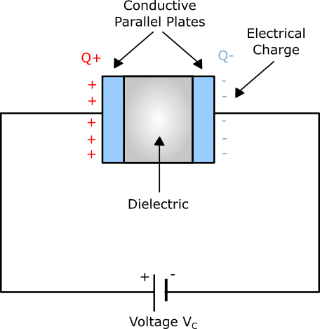
A capacitor stores electrical energy in an electric field. It consists of two conductive plates separated by an insulator (dielectric). Capacitors are used for energy storage, filtering and signal processing.
Structure and Function
Plates: Two conductors that hold equal and opposite charges.
Dielectric: An insulating material between the plates; it prevents charge flow while allowing the electric field to exist.
Electric field: Concentrated between the plates. Inside the conducting plates it is zero.
Capacitance
Capacitance\(C\) is the ratio of the charge \(q\) stored on each plate to the potential difference \(V\) between the plates:
\[
C = \frac{q}{V}
\]
Unit: farad (F), 1 F = 1 C/V.
For a parallel-plate capacitor (vacuum between plates):
\[
C = \frac{\varepsilon_0 A}{d}
\]
where \(A\) is the area of each plate (m²) and \(d\) the plate separation (m). With a dielectric, \(\varepsilon_0 \to \varepsilon_r\varepsilon_0\).
Energy Stored in a Capacitor
\[
U = \frac{1}{2} QV = \frac{1}{2} CV^2
\]
where \(Q\) is the charge on the plates (C) and \(V\) the voltage across them (V).
Electric Field in a Parallel-Plate Capacitor
Between the plates the field is (approximately) uniform:
\[
E = \frac{V}{d}
\]
Practical Applications
Energy storage: Rapid charge and discharge, e.g., flash photography, power supplies and backup systems.
Filtering: Smoothing voltage fluctuations in power supplies and selecting frequencies in audio and radio circuits.
Coupling / decoupling: Coupling capacitors pass AC while blocking DC; decoupling capacitors shunt unwanted AC (noise) to ground.
Timing: With resistors, capacitors set time constants in oscillators and pulse circuits.
RC Circuits
A resistor and a capacitor in series form an RC circuit, the simplest analog filter. When a voltage \(V_0\) is applied, the capacitor charges with the time constant\(\tau = RC\):
\[
V_C(t) = V_0 \left(1 - e^{-t/\tau}\right)
\]
After one time constant the capacitor reaches ≈ 63% of \(V_0\); after 5 time constants it is practically fully charged.
Taking the output across the capacitor gives a low-pass filter, taking it across the resistor gives a high-pass filter. Both have the cutoff frequency (gain \(1/\sqrt{2}\), i.e. −3 dB):
The hardware filters of EEG amplifiers are of this kind: the “time constant” setting of clinical EEG machines (e.g. 0.3 s) is the time constant of the high-pass filter, which corresponds to \(f_c = 1/(2\pi \cdot 0.3\,\mathrm{s}) \approx 0.53\) Hz. Digital filters are described in Filtering.
Coil
A coil (inductor) is a passive component that stores energy in a magnetic field when current flows through it. Coils are used for filtering, energy storage and signal processing.
Magnetic Field Generation
A current through a coil generates a magnetic field.
The field strength depends on the current, the number of turns and the core material (e.g., air, iron).
Inductance (\(L\))
Inductance is the property of a coil that opposes changes in current, analogous to inertia in mechanical systems. It is measured in henries (H), 1 H = 1 V·s/A.
The EMF induced in a coil is:
\[
V = -L \frac{\mathrm{d}I}{\mathrm{d}t}
\]
where \(L\) is the inductance (H) and \(\mathrm{d}I/\mathrm{d}t\) is the rate of change of current (A/s). The negative sign means that the induced EMF opposes the change in current (Lenz’s law).
Factors Affecting Inductance
Number of turns (\(N\)): more turns, larger inductance (\(\propto N^2\)).
Cross-sectional area (\(A\)): larger area, larger inductance.
Use: Analyzing current distribution in complex circuits.
Summary Table
Configuration
Current Relationship
Voltage Relationship
Example Components
Series
\(I_1 = I_2 = I_3\)
\(V = V_1 + V_2 + V_3\)
Resistors, capacitors, inductors
Parallel
\(I = I_1 + I_2 + I_3\)
\(V_1 = V_2 = V_3\)
Resistors, capacitors, inductors
Kirchhoff’s Law
Statement
Mathematical Form
KVL
Sum of voltage drops and rises in a loop is zero
\(\sum V = 0\)
KCL
Sum of currents entering a node equals sum of currents leaving
\(\sum I_{\text{in}} = \sum I_{\text{out}}\)
Energy Density
Energy density is the energy stored per unit volume in an electric or magnetic field. It describes how energy is distributed in space, e.g., in capacitors, inductors and electromagnetic waves.
Electric Field
\[
u_E = \frac{1}{2} \varepsilon_0 E^2
\]
where \(u_E\) is in J/m³ and \(E\) in V/m.
Magnetic Field
\[
u_B = \frac{1}{2\mu_0} B^2
\]
where \(u_B\) is in J/m³, \(\mu_0 = 4\pi\times 10^{-7}\) H/m is the permeability of free space and \(B\) is in T.
In both cases the energy density is proportional to the square of the field strength.
Total Energy Density
Where both fields exist (e.g., in electromagnetic waves):
Current density (\(\vec{J}\)) is a vector describing the flow of charge per unit area per unit time, measured in A/m².
Definition
For a uniform current perpendicular to a cross-section \(A\):
\[
J = \frac{I}{A}
\]
In general, the current through a surface \(S\) is the flux of \(\vec{J}\) through it:
\[
I = \int_S \vec{J} \cdot \mathrm{d}\vec{a}
\]
Vector Nature
Magnitude: charge flowing per unit area per unit time.
Direction: the direction of flow of positive charge (conventional current), even if the actual carriers (electrons) move the other way.
\[
\vec{J} = \rho \vec{v}
\]
where \(\rho\) is the (moving) charge density (C/m³) and \(\vec{v}\) the velocity of the charge carriers (m/s).
Direct Current (DC)
Direct current (DC) is the flow of electric charge in one direction only. It is produced by batteries, solar cells and DC generators.
Ohm’s Law: \(I = \frac{V}{R}\).
Current in series circuits: The current is the same at every point, before and after a resistor. A resistor converts energy but does not “use up” current.
Direction of Current
Electron flow: from the negative to the positive terminal of the battery.
Conventional current: drawn from the positive to the negative terminal (+ → −).
Voltage Drop
Definition: The voltage drop \(\Delta V\) across a resistor is the decrease in electric potential as charge flows through it.
Energy dissipation: The potential energy lost by the charges is converted to heat.
Electrical Power in DC Circuits
\[
P = I \Delta V
\]
where \(\Delta V\) is the voltage drop across the component (V) and \(I\) the current through it (A). Using \(\Delta V = IR\):
\[
P = I^2 R = \frac{(\Delta V)^2}{R}
\]
Units: watts, 1 W = 1 J/s.
Energy in DC Circuits
The energy transferred when a charge \(Q\) moves through a potential difference \(V\) is \(W = VQ\); for constant power over a time \(t\), \(W = Pt\).
Alternating Current (AC)
Alternating current (AC) periodically reverses direction, unlike DC. It is the standard form of electricity for power distribution in homes and industry.
A magnetic field (B-field) is a vector field describing the magnetic influence on moving charges, electric currents and magnetic materials. It governs the interactions between magnets, currents and charged particles.
Units and Relationships
Magnetic flux density (\(B\)):
Unit: tesla (T), \(1\,\text{T} = 1\,\frac{\text{N}}{\text{A}\cdot\text{m}} = 1\,\frac{\text{kg}}{\text{A}\cdot\text{s}^2}\)
Represents the strength and direction of the magnetic field.
Magnetic field strength (\(H\)):
Unit: amperes per meter (A/m).
In vacuum, \(B = \mu_0 H\), where \(\mu_0 = 4\pi\times 10^{-7}\) T·m/A.
Sources of Magnetic Fields
Moving electric charges: e.g., electrons in a current-carrying wire.
Intrinsic magnetic moments: elementary particles such as electrons have a magnetic moment due to spin.
Permanent magnets: materials such as iron, cobalt and nickel can be permanently magnetized.
Electromagnetism is the interaction between electric and magnetic fields.
Practical Implications
Electric fields: capacitors, electronics, electrostatic applications.
Magnetic fields: motors, generators, MRI machines, data storage.
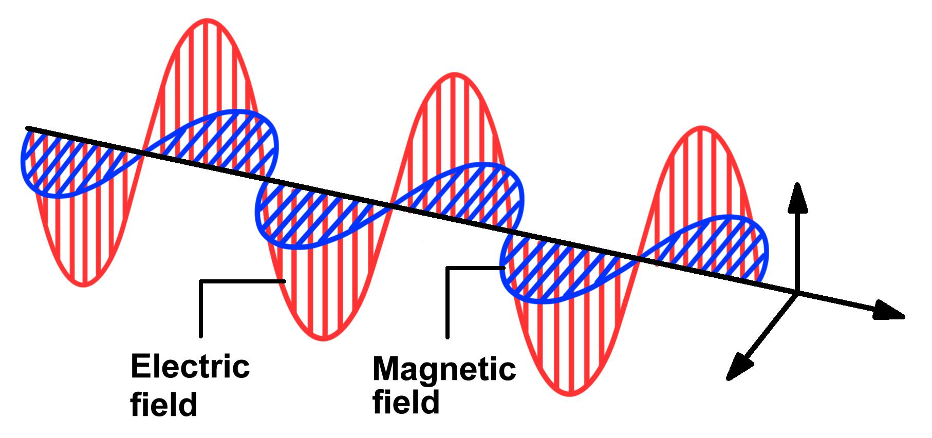
Electromagnetic waves: light, radio waves and X-rays are solutions of Maxwell’s equations, in which \(\vec{E}\) and \(\vec{B}\) propagate together through space.
Visualization
Electric field lines: radial for point charges, parallel for uniform fields.
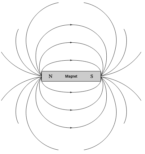
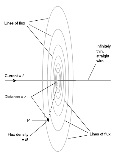
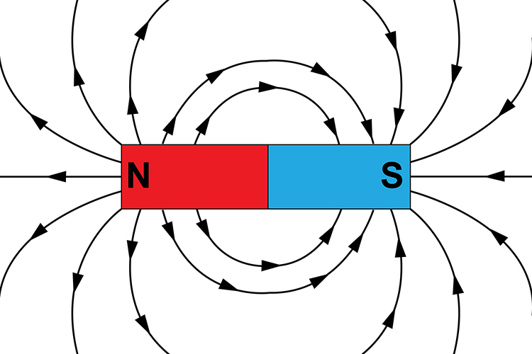
Magnetic field lines: circles around currents; closed loops running from N to S outside a magnet.
Lorentz Force
The total force on a particle with charge \(q\) moving with velocity \(\vec{v}\) in electric field \(\vec{E}\) and magnetic field \(\vec{B}\) is:
Magnetic force: \(\vec{F}_m = q(\vec{v} \times \vec{B})\)
The magnitude of the magnetic force is:
\[
F_m = qvB\sin(\theta)
\]
where \(\theta\) is the angle between \(\vec{v}\) and \(\vec{B}\). The magnetic force does no work on the particle, since it is always perpendicular to \(\vec{v}\).
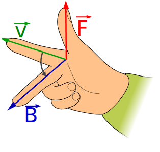
Direction of the Magnetic Force (right-hand rule, for positive \(q\))
Point your fingers along the velocity \(\vec{v}\).
Curl them toward the magnetic field \(\vec{B}\).
Your thumb points along the force \(\vec{F}_m\) (reverse it for a negative charge).
This shows that the magnetic force is orthogonal to both \(\vec{v}\) and \(\vec{B}\).
Magnetometer
A magnetometer measures the strength and direction of a magnetic field. One of the most sensitive types is the SQUID (Superconducting Quantum Interference Device), which can detect extremely weak fields.
Magnetic Field Properties
No magnetic monopoles: No isolated magnetic charges have ever been observed. Magnetic fields are produced by currents and dipoles, each with a north (N) and a south (S) pole.
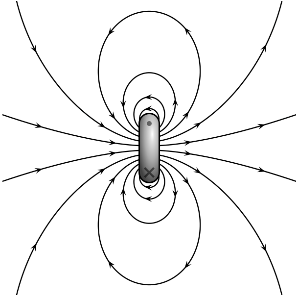
Closed loops: Magnetic field lines never start or end. Outside a magnet they run from the N pole to the S pole; inside the magnet they continue from S to N.
Magnetic Field Models
H-field (magnetic pole model)
Analogy to the electric field: + corresponds to the N pole and − to the S pole.
Field lines: drawn like electric field lines, from the N pole to the S pole.
B-field (Amperian loop model)
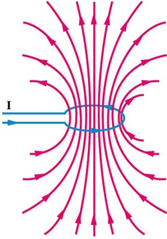
Current loops: The B-field (magnetic flux density) is generated by current loops. A small loop with current \(I\) and area \(A\) acts as an elementary magnetic dipole.
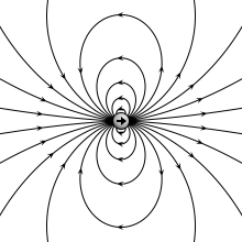
Magnetic dipole: As the loop radius shrinks (at constant moment), its field becomes identical to that of an idealized point dipole.
Magnetic Dipoles
A magnetic dipole is a tiny current loop that produces a field similar to a bar magnet. Its field is characterized by the dipole moment, a vector pointing from the S pole to the N pole.
Magnetic Moment
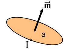
The magnetic moment\(\vec{m}\) quantifies the strength and orientation of a magnet or current loop. It is a vector quantity; its SI unit is A·m².
Magnetic Moment of a Current Loop
\[
\vec{m} = I \vec{A}
\]
where \(\vec{A}\) has the magnitude of the loop area and a direction perpendicular to the loop plane (given by the right-hand rule).
Torque and Force on a Magnetic Moment
In a magnetic field, a magnetic moment experiences a torque that tends to align it with the field:
\[
\vec{\tau} = \vec{m} \times \vec{B}
\]
In a non-uniform field it also experiences a force:
\[
\vec{F} = \nabla (\vec{m} \cdot \vec{B})
\]
where \(\nabla\) is the gradient operator and \(\vec{m} \cdot \vec{B} = mB \cos(\theta)\), with \(\theta\) the angle between \(\vec{m}\) and \(\vec{B}\).
Faraday’s Law of Induction
Faraday’s law states that a changing magnetic field induces an electric field, which can drive an electromotive force (EMF) in a circuit. This is the principle behind generators and transformers.
where: \(\mathcal{E}\) is the induced EMF (V), \(N\) is the number of turns, \(\Delta \Phi\) is the change in magnetic flux (Wb), \(\Delta t\) is the time interval (s).
Magnetic Flux and Induction
The magnetic flux through a surface (uniform field, flat surface) is:
\[
\Phi = \vec{B} \cdot \vec{A} = BA \cos(\theta)
\]
where: \(\vec{B}\) is the magnetic field (T), \(\vec{A}\) is the area vector (m²), perpendicular to the surface, \(\theta\) is the angle between \(\vec{B}\) and \(\vec{A}\).
Right-Hand Rule for Current and Magnetic Field
Current direction: conventional current flows from + to −.
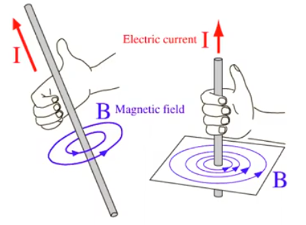
Field direction: grip the wire with your right hand, thumb along the current. Your fingers curl in the direction of the magnetic field lines.
Magnetic Field of a Long Straight Wire
\[
B = \frac{\mu_0 I}{2\pi r} = 2 \times 10^{-7} \frac{I}{r} \quad (\text{in vacuum or air})
\]
where \(B\) is in T, \(I\) is the current (A) and \(r\) is the distance from the wire (m).
Force on a Current-Carrying Wire in a Magnetic Field
\[
F = IlB \sin(\theta)
\]
where \(F\) is the force (N), \(I\) the current (A), \(l\) the length of wire in the field (m), \(B\) the field (T) and \(\theta\) the angle between the wire and the field.
The force is maximal when the wire is perpendicular to the field (\(\theta = 90^{\circ}\)).
Magnetic Properties of Materials
Permeability (\(\mu\)): how easily a material can be magnetized.
Relative permeability (\(\mu_r\)): \(\mu = \mu_r \mu_0\). For a vacuum, \(\mu_r = 1\).
Retentivity: the ability of a material to retain magnetization after the external field is removed.
Core saturation: the maximum flux density a magnetic core can reach; beyond it, increasing the current barely increases the flux.
Materials are classified by their response to a magnetic field:
Type
Relative permeability
Behavior
Examples
Diamagnetic
\(\mu_r\) slightly < 1
weakly repelled by a magnetic field
water, biological tissue, copper
Paramagnetic
\(\mu_r\) slightly > 1
weakly attracted; no magnetization without external field
aluminum, oxygen
Ferromagnetic
\(\mu_r \gg 1\) (up to 10⁵)
strongly attracted; can be permanently magnetized
iron, nickel, cobalt, mu-metal
Biological tissue has \(\mu_r \approx 1\): the head is magnetically transparent, so the magnetic field of brain currents passes through the skull and scalp without distortion. Ferromagnetic alloys with high permeability (mu-metal) are used in magnetically shielded rooms for MEG.
Maxwell’s Equations
Maxwell’s equations are four fundamental laws describing how electric and magnetic fields are generated and interact. They underlie classical electromagnetism, optics and electric circuits.
Meaning: Magnetic fields are generated by electric currents and by changing electric fields (basis of electromagnetic waves).
\(\vec{J}\): current density; \(\mu_0\): permeability of free space.
Integral form: relates the fields on the boundary of a region (closed surface or loop) to the sources inside it; used for the field over extended regions, especially with symmetry.
Differential form: local relations between the fields and their sources at each point in space.
The two forms are equivalent and can be converted into each other with the divergence and curl theorems.
\(A\): closed surface enclosing the volume \(V\) (a closed surface integral, written \(\oint_A\)) \(\mathbf{F}\): vector field (\(\mathbf{E}\) or \(\mathbf{B}\))
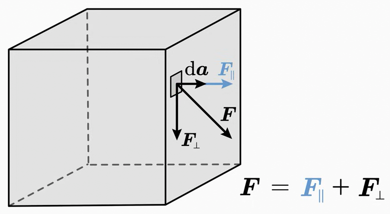
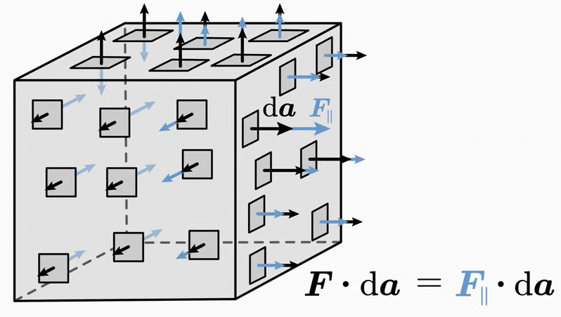
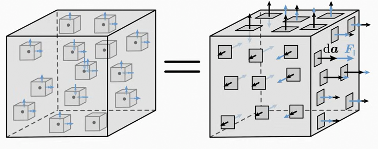
\(\mathrm{d}\mathbf{a}\): infinitesimal surface element of \(A\); its magnitude is the area of that small piece of surface and its direction points out of the surface.
The dot product removes the part of \(\mathbf{F}\) tangent to the surface and keeps only the component perpendicular to it. Summing over the whole surface gives the flux\(\phi\), the integral of a vector field through a surface. It tells how much of the field flows out of (or into) the surface \(A\):
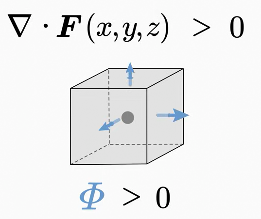
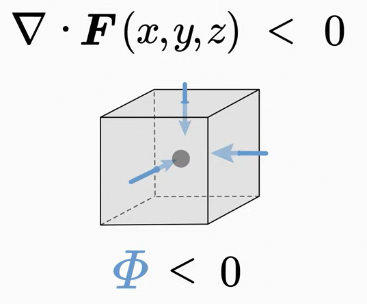
\(\nabla \cdot \mathbf{F}\) is the divergence of the field, a scalar function: \(\nabla \cdot \mathbf{F}(x, y, z) = \mathtt{scalar}\).
If \(\nabla \cdot \mathbf{F} > 0\) at a point, there is a source of the field there. If the surface encloses this source, the flux is positive: the field flows out of the surface.
If \(\nabla \cdot \mathbf{F} < 0\) at a point, there is a sink of the field there. If the surface encloses this sink, the flux is negative: the field flows into the surface.
If \(\nabla \cdot \mathbf{F} = 0\), inflow and outflow cancel, or there is no flow.
Summing the divergence over every point of \(V\) gives the left-hand side. Therefore:
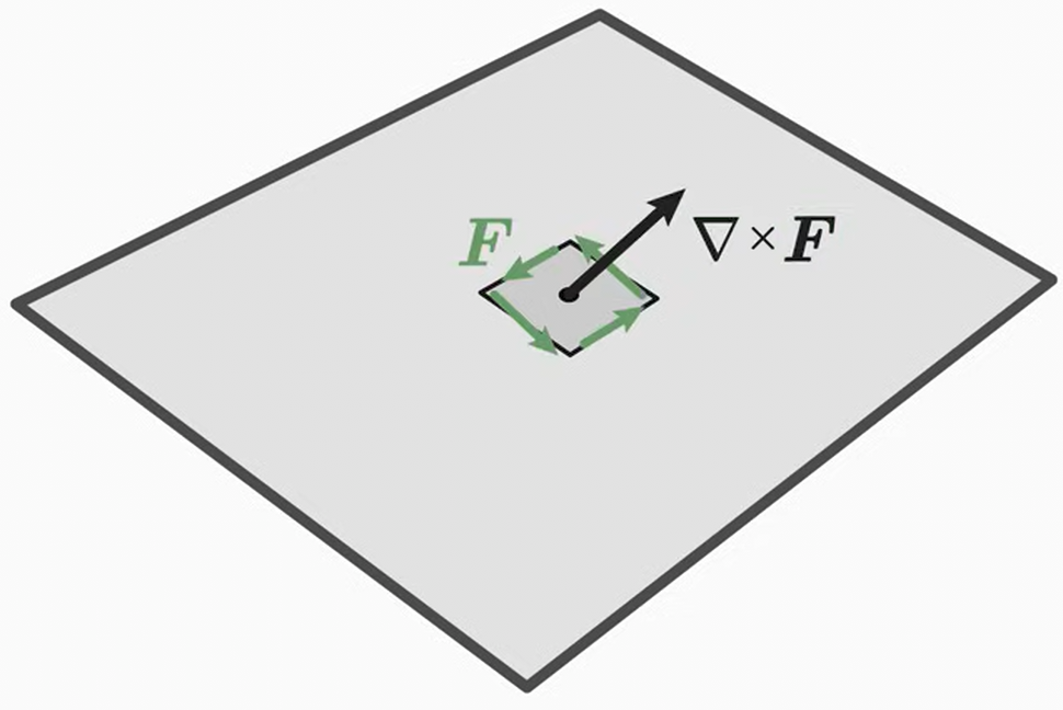
The curl describes how much the field rotates around a point.
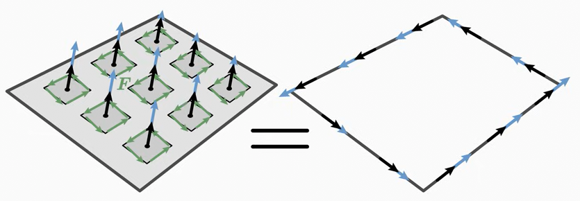
The dot product \((\nabla \times \mathbf{F}) \cdot \mathrm{d}\mathbf{a}\) keeps only the part of the curl perpendicular to the surface; these contributions are summed over \(A\).
The total curl of \(\mathbf{F}\) over the surface \(A\) equals the circulation of \(\mathbf{F}\) along the edge \(L\) of that surface.
\(\nabla \cdot \mathbf{E} = 0 \Rightarrow \rho = 0\): no charge at that point (or charges cancel).
Electric charges are the sources (+) and sinks (−) of the electric field.
In a region with no charge, as much field enters a small volume as leaves it. A positive charge makes the field arrows leave the region, a negative charge makes them enter.
2nd Maxwell’s equation (Gauss’s law for magnetism)
Since this holds for every volume \(V\), the integrand must vanish everywhere.
Differential form:
\[
\nabla \cdot \mathbf{B} = 0
\]
The divergence of the magnetic field is always zero: there are no sources or sinks of \(\mathbf{B}\) (magnetic monopoles). The field also continues inside a magnet, so magnetic field lines always form closed loops.
3rd Maxwell’s equation (Maxwell-Faraday equation, Faraday’s law of induction)
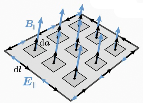
Right-hand side: the rate of change of the magnetic flux \(\phi_m\) through the surface \(A\) bounded by \(L\). The faster the flux changes, the stronger the induced circulating electric field. The minus sign (Lenz’s law) means that the induced field opposes the change in flux: if the flux increases, the induced EMF drives a current whose field reduces the flux, and vice versa.
A changing magnetic field induces a circulating electric field. (Conversely, a changing electric field produces a magnetic field; see the 4th equation.)
Differential form: with Stokes’ theorem on the left-hand side and (for a fixed surface) moving the time derivative inside the integral on the right:
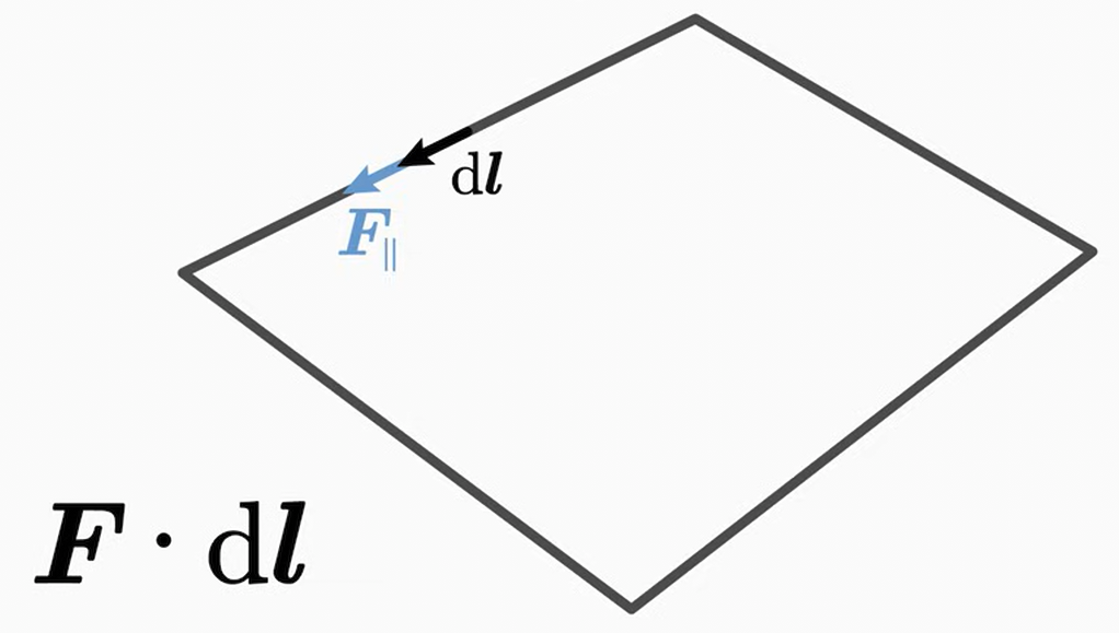
Symbols: \(\oint_L\): line integral over a closed loop (e.g., a circle) \(\vec E\): electric field \(\mathrm{d}\vec{l}\): small element of the loop \(\vec E \cdot \mathrm{d}\vec{l}\): dot product, maximal when aligned and zero when perpendicular; the component of \(\vec E\) along the loop \(\vec B\): magnetic field \(\mathrm{d}\vec{a}\): small element of the surface \(A\) bounded by the loop \(\vec B \cdot \mathrm{d}\vec{a}\): how much of \(\vec B\) passes through that element \(\mathrm{d}/\mathrm{d}t\): rate of change in time
Electromagnetic induction: a changing magnetic flux through a loop induces an EMF (and so a current) in it. The EMF around a wire loop equals the negative rate of change of the magnetic flux through the loop. A magnet moving through a coil generates a voltage (EMF) across the coil.
Left-hand side: the circulation of the magnetic field along the closed loop \(L\) (the “magnetic voltage”), \(U_m = \oint_L \mathbf{B} \cdot \mathrm{d}\mathbf{l}\).
First term on the right: the electric current \(I_{\text{enc}}\) passing through the surface \(A\) bounded by \(L\).
Second term on the right (Maxwell’s displacement term): the rate of change of the electric flux through \(A\). A changing electric field acts like a current in producing a magnetic field.
Writing \(I_{\text{enc}} = \int_A \mathbf{J} \cdot \mathrm{d}\mathbf{a}\) and applying Stokes’ theorem gives the differential form:
where: \(\vec{B}\) is the magnetic field, \(d\vec{s}\) is the infinitesimal element of the loop, \(\mu_0\) is the magnetic constant (\(4\pi\times 10^{-7}\) N/A²), \(I_{\text{enc}}\) is the current enclosed by the loop.
Magnetic Interaction Between Current-Carrying Wires
Same direction: parallel wires carrying current in the same direction attract each other.
Opposite directions: parallel wires carrying current in opposite directions repel each other.
Magnetic Field of a Straight Wire
For a wire carrying current \(I\), take a circular loop of radius \(r\) around it:
Angle: \(\vec{B}\) is tangent to the circle, so \(\theta = 0^{\circ}\) between \(\vec{B}\) and \(d\vec{s}\) and \(\cos(\theta) = 1\).
Line integral: \(\oint B \cos(\theta) \, ds = B \oint ds = B (2 \pi r)\)
Induction: A changing magnetic field (flux) induces an electric field, which can drive a current in a conductor.
Lenz’s law: The induced current flows in the direction that opposes the change in flux that produced it.
Steady current: A steady current produces a constant magnetic field, which induces no current in a stationary loop. Current is induced only when the flux changes.
Flux
Flux measures how many field lines pass through an area. It depends on:
the strength of the field,
the area of the surface,
the angle between the field and the surface normal (flux is zero when the field is parallel to the surface).
Electric flux\(\phi_E\) through a small patch \(\mathrm{d}S\):
\[
\mathrm{d}\phi_E = E \, \mathrm{d}S \cos(\theta)
\]
where \(\theta\) is the angle between the field and the normal to the patch. Summing over a closed surface:
The dot product accounts for the angle between the field and the patch. Gauss’s law:
\[
\oint \vec E \cdot \mathrm{d}\vec A = \frac{q}{\varepsilon_0}
\]
where \(q\) is the enclosed charge and \(\varepsilon_0\) the permittivity of free space. When \(E\) is constant and perpendicular to the surface (by symmetry), this reduces to \(E A = q/\varepsilon_0\).
Magnetic flux through a closed surface is zero, since every line that leaves a surface returns through it:
\[
\oint \vec B \cdot \mathrm{d}\vec A = 0
\]
Through an open surface (e.g., a loop), for a uniform field:
\[
\Phi_B = B A \cos(\theta)
\]
where: \(\Phi_B\) is the magnetic flux (weber, Wb), \(B\) is the magnetic field strength (T), \(A\) is the area of the loop (m²), \(\theta\) is the angle between the field and the normal to the loop.
For a loop perpendicular to the field (\(\theta = 0^{\circ}\)): \(\Phi_B = BA\).
When the loop rotates, the rate of change \(\mathrm{d}\Phi_B/\mathrm{d}\theta = -BA\sin\theta\) is zero at \(\theta = 0^{\circ}\) (flux is at its maximum) and largest in magnitude at \(\theta = 90^{\circ}\) (flux passes through zero).
A changing magnetic flux induces an EMF (Faraday’s law); the minus sign expresses Lenz’s law:
Example: a loop rotating at constant angular velocity \(\omega\) in a uniform field has \(\theta = \omega t\), so \(\Phi_B = BA\cos(\omega t)\) and \(\mathcal{E} = BA\omega\sin(\omega t)\). The plot shows the flux (normalized to \(BA\)) and the EMF (normalized to \(BA\omega\)) as functions of the angle.
The EMF is largest when the flux passes through zero (90°, 270°) and zero when the flux is at its maximum or minimum: the induced voltage depends on the rate of change of the flux, not on the flux itself. This is the principle of electric generators, and also why a moving conductor (e.g. a cable swinging in the magnetic field of a power line) picks up interference.
Electric Vector Field
For each point in space, a vector with magnitude and direction can be assigned.
Example: two charges with \(q_+ = 3\,\vert q_- \vert\) in the plane \(z = 0\):
\(q_+\) is located at \((0, -d, 0)\),
\(q_-\) is located at \((0, d, 0)\).
In units of \(q_+/(4\pi\varepsilon_0)\) the field is:
The field in the plane \(z = 0\) (positive charge in red, negative in blue; colors show the field strength):
d =1.0# field of q₊ at (0, -d) and q₋ = -q₊/3 at (0, d), in units of q₊/(4πε₀)functionefield(x, y) E =Point2f(0, 0)for (q, y0) in ((1.0, -d), (-1/3, d)) rv =Point2f(x, y - y0) E += q * rv /norm(rv)^3endreturn Eendfig, ax, pl =streamplot(efield, -3..3, -3..3; colormap =:viridis, figure = (size = (700, 650),), axis = (ax_style_small..., xticks =LinearTicks(7), aspect =DataAspect(), title ="q₊ = 3|q₋|", xlabel ="x / d", ylabel ="y / d"))scatter!(ax, [0, 0], [-d, d]; color = [:red, :blue], markersize =18)fig
All field lines ending on the negative charge start on the positive charge, but most lines from the stronger positive charge go to infinity: far from the charges, the field looks like that of a single charge \(q_+ + q_- = \frac{2}{3} q_+\).
Electromagnetism of EEG and MEG
Quasi-static approximation
Brain signals contain frequencies below ≈ 1 kHz. At these frequencies, the wavelength of electromagnetic waves (hundreds of kilometers) is enormous compared with the head, and in head tissues the capacitive (displacement) currents and inductive effects are negligible compared with the conduction currents. The time derivatives in Maxwell’s equations can therefore be neglected (quasi-static approximation):
the electric field can be written as \(\mathbf{E} = -\nabla V\) (a potential exists, which EEG measures),
the fields at any instant depend only on the currents at that instant: there is no delay between the brain source and the sensors, and EEG/MEG signals are instantaneous mixtures of the source activities,
the measured signals are linear in the source strengths, which is the basis of forward and inverse modeling (see Brain electric model).
Primary and volume currents
Synchronous postsynaptic currents in the apical dendrites of many parallel pyramidal neurons form the primary current\(\mathbf{J}^p\). It is closed by volume currents (return currents) driven by the electric field in the conducting tissue:
where \(\sigma\) is the conductivity of the tissue (≈ 0.33 S/m for brain and scalp, much lower for the skull). A small patch of active cortex is modeled as a current dipole\(\mathbf{Q}\) (unit: A·m), pointing along the dendrites, i.e. perpendicular to the cortical surface. Evoked responses correspond to dipole strengths of the order of 10–100 nA·m, which require the synchronous activity of a large population of neurons (tens of thousands or more in a few square centimeters of cortex): currents of single neurons are far too weak to be measured outside the head, and currents of neurons that are not aligned or not synchronous cancel each other.
EEG: the electric potential
In an infinite homogeneous conductor, the potential of a current dipole \(\mathbf{Q}\) at \(\mathbf{r}_0\) is:
This is the dipole potential of electrostatics with \(\varepsilon_0\) replaced by \(\sigma\). EEG measures the volume currents: the potential they produce on the scalp. In a real head, the low conductivity of the skull attenuates and spatially smears the potential.
MEG: the magnetic field
The magnetic field of a current distribution is given by the Biot–Savart law. For a current dipole:
The volume currents also produce a magnetic field. In a spherically symmetric conductor, however, they do not contribute to the field component normal to the surface (radial), and the total field outside the sphere does not depend on the conductivities. Because tissues are magnetically transparent (\(\mu_r \approx 1\)) and MEG is little affected by the skull, the MEG field is less distorted than the EEG potential.
Example: a tangential current dipole of 10 nA·m (pointing along \(x\)) in an infinite homogeneous conductor, and the EEG potential and the normal magnetic field \(B_z\) (from the primary current, as in a sphere) in a plane 3 cm above it:
# conductivity (S/m), μ₀/4π (T·m/A)σ =0.33μ0_4π =1e-7# 10 nA·m tangential dipole at the origin, sensors 3 cm above itQ = [10e-9, 0, 0]h =0.03xs =range(-0.08, 0.08; length =161)V = [dot(Q, [x, y, h]) / (4π * σ *norm([x, y, h])^3) for x in xs, y in xs]Bz = [μ0_4π *cross(Q, [x, y, h])[3] /norm([x, y, h])^3 for x in xs, y in xs]println("maximum potential: ",round(1e6*maximum(abs.(V)); digits =2), " μV")println("maximum magnetic field: ",round(1e15*maximum(abs.(Bz)); digits =0), " fT")
maximum potential:      1.03 μV
maximum magnetic field: 428.0 fT
The EEG potential has a positive and a negative extremum along the dipole direction, and the dipole lies between them.
The magnetic field pattern is rotated by 90°: the extrema lie on both sides of the dipole, and the dipole lies between them, perpendicular to the line connecting them (right-hand rule).
The magnetic field is in the range of hundreds of femtotesla, ≈ \(10^9\) times weaker than the Earth’s magnetic field.
A radial dipole (pointing towards the sensors, i.e. along \(z\)) produces no normal magnetic field, because \(\mathbf{Q} \times (\mathbf{r} - \mathbf{r}_0)\) has no \(z\) component:
Qr = [0, 0, 10e-9]Bz_radial = [μ0_4π *cross(Qr, [x, y, h])[3] /norm([x, y, h])^3 for x in xs, y in xs]println("maximum B_z of a radial dipole: ",maximum(abs.(Bz_radial)), " T")
maximum B_z of a radial dipole: 0.0 T
In a spherical conductor, radial dipoles produce no magnetic field outside the head at all. MEG is therefore most sensitive to tangential sources (in the walls of sulci), EEG to both tangential and radial sources (on the crowns of gyri) — the two methods are complementary.
Magnitudes of magnetic fields
Source
Magnetic field
MRI scanner
1.5–7 T
Earth’s magnetic field
≈ 50 μT
Urban environmental noise
≈ 1 nT – 1 μT
Heart (magnetocardiography)
≈ 10–100 pT
Spontaneous brain activity (e.g. alpha)
≈ 0.1–1 pT
Evoked brain responses
≈ 10–100 fT
SQUID sensor noise
≈ 2–5 fT/√Hz
Measuring femtotesla fields in the presence of noise many orders of magnitude larger requires sensitive sensors (SQUIDs, optically pumped magnetometers), magnetically shielded rooms and noise-suppression methods (gradiometers, SSP, SSS):
magnetometers measure one component of the field (unit: fT),
gradiometers measure the difference of the field between two nearby coils, i.e. its spatial gradient (unit: fT/cm). Distant noise sources produce nearly uniform fields, which cancel, while the steep gradients of nearby brain sources are retained.
Hämäläinen M, Hari R, Ilmoniemi RJ, Knuutila J, Lounasmaa OV. Magnetoencephalography — theory, instrumentation, and applications to noninvasive studies of the working human brain. Reviews of Modern Physics. 1993;65(2):413–97.
Griffiths DJ. Introduction to Electrodynamics. 4th ed. Cambridge University Press; 2017.
Nunez PL, Srinivasan R. Electric Fields of the Brain: The Neurophysics of EEG. 2nd ed. Oxford University Press; 2006.
Sarvas J. Basic mathematical and electromagnetic concepts of the biomagnetic inverse problem. Physics in Medicine and Biology. 1987;32(1):11–22.