Introduction to Signal Theory

using NeuroAnalyzer
using CairoMakie
CairoMakie.activate!(type = "png")
using StatsKit
using FFTW

A practical guide to signals, systems, and the mathematical foundations of neural signal processing.

System

A system transforms an input signal into an output signal:

\[ \text{input} \rightarrow \text{H} \rightarrow \text{output} \]

For continuous signal: \(y[t] = H(x[t])\). For a discrete signal: \(y[n] = H(x[n])\).

The snippet below overlays a continuous sine with its sampled (discrete) version:

t = linspace(0, 2pi, 100)
s = sin.(t)

fig, ax = lines(t, s)
stem!(ax, t[1:2:end], s[1:2:end])
fig

Linear Systems

A system is linear if it obeys two properties simultaneously:

1. Additivity: \(H(x_1[n] + x_2[n]) = y_1[n] + y_2[n]\)
2. Homogeneity: \(H(a \times x_1[n]) = a \times y_1[n]\)

Time-Invariant Systems

A time-invariant system behaves identically regardless of when the input arrives: a temporal shift at the input produces an equal shift at the output.

\[ x[n] \rightarrow H \rightarrow y[n] \Leftrightarrow x[n - 1] \rightarrow H \rightarrow y[n - 1] \]

LTI Systems

A system that is both linear and time-invariant is an LTI system. Most real-world systems are approximated as LTI - the model is tractable and often accurate enough for practical use.

Memory-less Systems

A system is memory-less when its output at time \(n\) depends only on its input at that same instant:

Memory-less system:

\[ y[n] = x[n]^2 \]

System that has memory:

\[ y[n] = x[n - 1] \]

Causal Systems

A causal system’s output depends only on present and past inputs - never future ones.

Causal system:

\[ y[n] = x[n] - 2 \times x[n - 1] \]

Non-causal:

\[ y[n] = x[n + 3] \]

Causal system cannot anticipate future inputs.

Example: A 3-sample moving average using samples \(n-1\), \(n\) and \(n+1\) is non-causal - it requires a future value.

Signals

A signal is any quantity measured at regular intervals. Signals are either continuous (defined at every instant) or discrete (sampled at fixed intervals).

Special Signals

Unit Impulse

The unit impulse, also known as the delta function or Dirac delta function, is a fundamental concept in signal processing and systems analysis. In discrete-time systems, it is defined as follows:

Mathematical Definition

\[ \delta[n] = \begin{cases} 1 & \text{if $n = 0$}\\ 0 & \text{otherwise} \end{cases} \]

where:
\(\delta[n]\) is the unit impulse function,
\(n\) is the discrete-time index.

A unit spike at \(n = 0\). Any discrete signal can be expressed as a weighted sum of shifted impulses.

Impulse Response:

In linear time-invariant (LTI) systems, the impulse response \(h[n]\) is the output of the system when the input is a unit impulse \(\delta[n]\). This response characterizes the system completely.

Unit step function

The unit step function, often denoted as \(u[n]\), is a fundamental concept in discrete-time signal processing.

Mathematical Definition

\[ u[n] = \begin{cases} 1 & \text{if $n \geq 0$}\\ 0 & \text{otherwise} \end{cases} \]

where:
\(u[n]\) is the unit step function,
\(n\) is the discrete-time index.

Equivalently, a running sum of shifted deltas:

\[ u[n] = \sum_{k=0}^{\infty} \delta[n - k] = \sum_{k=-\infty}^{n} \delta[k] \]

Time series (TS) vs. signal

\[ \text{time series} = \text{signal} + \text{noise} \]

A time series is the raw sequence of samples; a signal is the meaningful component within it. In EEG, the signal is voltage (µV) varying over time (ms).

Key Terminology

Sampling rate: Samples per second. Also the number of zero-crossings per second × 0.5.

\[ f = 1 / T \]

where:
\(f\) is the frequency: cycles per second (Hz),
\(T\) is the period: length of one period (cycle) (s).

Sampling interval: Time between consecutive samples: \(1 / f\).

Fundamental frequency: The lowest frequency component present.

Harmonics: Integer multiples of the fundamental frequency.

Octave: A doubling in frequency.

Dominant frequency: The component with the highest amplitude.

Elementary Signal Types

x = -1:0.1:1

# unit step
us = Int64.(x .>= 0)

# reversed unit step
reversed_us = Int64.(x .<= 0)

# use US to gate a signal on/off
new_signal = signal .* us

# impulse
imp = Int64.(x .== 0)

# ramp
ramp = Int64.(x .* us)

# quadratic
quad = Int64.(x .^ 2 .* us)

# exponential (x >= 0)
y = exp.(-x)

# half-wave rectifier
hwr = y .* Int64.(y .> 0)

# full-wave rectifier
fwr = abs.(y)

Signal Classification

Every signal can be categorized along the following axes:

1. Periodic or Non-periodic
2. Odd (= asymmetric) or Even (= symmetric) or Neither
3. Power or Energy
4. Real or Complex
5. Continuous Time or Discrete Time
6. Random (stochastic) or Deterministic
7. Linear or Non-linear
8. Causal (future inputs do not modify the signal) or Non-causal
9. Stable or Unstable (erratic and extreme behaviors)

Periodic signal: Repeats with the smallest period \(T\) satisfying \(s(t + T) = s(t)\). Its frequency is a rational number.

Even signal: Symmetric about the origin: \(s(t) = s(-t)\).

Odd signal: Anti-symmetric about the origin: \(s(t) = -s(-t)\).

Processing Operations

Amplification: \(k \times s(t)\) for \(k > 1\) - scales magnitude up.

Attenuation: \(k \times s(t)\) for \(0 < k < 1\) - scales magnitude down.

Shifting: \(s(t - t_0)\) - shifts right; \(s(t + t_0)\) - shifts left.

Scaling: \(s(k \times t)\) squeezes the signal when \(0 < k < 1\) and stretches when \(k > 1\).

Combination: Signals can be added \(a(t) + a(t)\) or multiplied \(a(t) \times a(t)\) sample-by-sample.

Feedback

A feedback loop routes part of a system’s output back to its input. Feedback can stabilise an unstable system - but it can equally introduce instability if the loop gain is not carefully managed. Real-world designs must be analyzed to verify stability before deployment.

Signal Parameters

Any oscillation is fully characterized by three quantities:

1. Frequency - how fast does it oscillate?
2. Power - how strong is it?
3. Phase - when does the cycle start? (the amplitude at \(t = 0\))

Amplitude

Amplitude measures the extent of oscillation. Four common measures:

1. Peak amplitude \(\hat{u}\) - refers to the maximum absolute value of a signal’s deviation from its baseline (or zero, if the baseline is zero).
2. Peak-to-peak amplitude \(2\hat{u}\) - is the difference between the maximum positive peak and the minimum negative peak of a signal.
3. RMS amplitude for pure sinusoidal signal: \(\hat{u}/\sqrt{2}\).
4. Wave period - a measure of time, not amplitude.

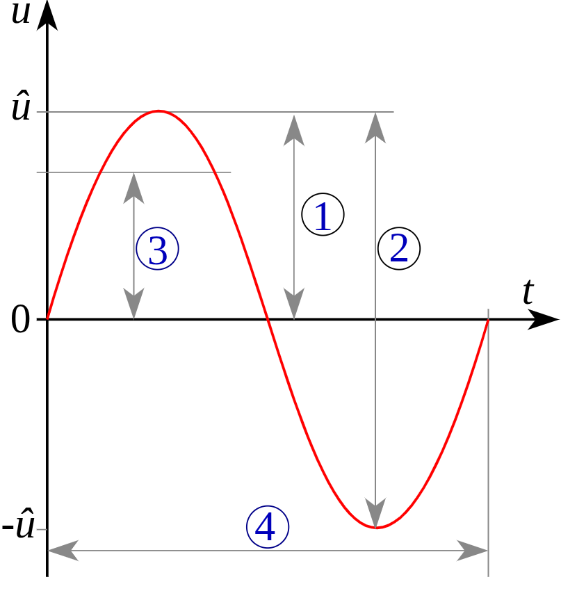
Peak amplitude measures the strength of individual EEG components (e.g., amplitude of an ERP or spike). It is useful for detecting abnormal spikes (e.g., epileptic discharges).

Peak-to-peak amplitude reflects the overall variability of the EEG signal (e.g., alpha or beta wave amplitude). It is used to assess signal-to-noise ratio or amplitude modulation in brain rhythms.

RMS amplitude of a non-pure sinusoidal signal is a statistical measure of the magnitude of a varying signal, such as EEG data. It calculates the square root of the average of the squared values of the signal over a given time window. RMS amplitude provides a single value that represents the effective amplitude of the signal, accounting for both positive and negative fluctuations.

For a discrete signal \(s\) with \(N\) samples:

\[ \text{RMS Amplitude} = \sqrt{\frac{1}{N} \sum_{i=1}^{N} s_i^2} \]

where:
\(s_i\) is the amplitude of the signal at sample \(i\),
\(N\) is the total number of samples in the signal.

Phase & Time Shift

Phase is 0° when the sine wave’s peaks align with the edges of the analysis window - matching a cosine shape. Other phases are measured relative to this. A rightward time shift decreases phase; a leftward shift increases it.

The general sine wave is:

\[ y = a \times \sin(2\pi \times f \times t + \theta) \]

Replacing \(t\) with \(t + t_0\) shifts the waveform in time, which is equivalent to adding a phase offset.

t = 0:0.01:2pi
s1 = sin.(2pi * 0.5 .* t)
# shifted left in time
s2 = sin.(2pi * 0.5 .* (t .+ 0.5))
# shifted right in time
s3 = sin.(2pi * 0.5 .* (t .- 0.5))

fig, ax = lines(t, s1, color = :black, label = "original")
lines!(ax, t, s2, color = :red, label = "t + 0.5")
lines!(ax, t, s3, color = :blue, label = "t - 0.5")
axislegend(ax, position = :rt)
fig

Noise

White noise: Equal power at all frequencies (flat spectrum). Can be uniformly or normally distributed.

1. normal distributed
2. uniformly distributed

Gaussian white noise:

fs = 100
t = 0:1/fs:10
gwn = randn(length(t))
NeuroAnalyzer.plot(t, gwn, title = "Gaussian White Noise")

Amplitude histogram:

plot_histogram(gwn,
               title  = "Amplitude Distribution",
               xlabel = "Amplitude",
               ylabel = "Count",
               draw_median = false)

PSD:

# Fourier transform
X = ftransform(gwn)
# f will contain vector of frequencies
f, _ = freqs(gwn, fs)
plot_psd(f, X.p, flim = (1, 40))

Uniform white noise:

fs = 100
t = 0:1/fs:10
uwn = rand(length(t))
NeuroAnalyzer.plot(t, uwn, title = "Uniform White Noise")

Amplitude histogram:

plot_histogram(uwn,
               title  = "Amplitude Distribution",
               xlabel = "Amplitude",
               ylabel = "Count",
               draw_median = false)

PSD:

# Fourier transform
X = ftransform(uwn)
# f will contain vector of frequencies
f, _ = freqs(uwn, fs)
plot_psd(f, X.p, flim = (1, 40))

Pink noise: Power decreases with increasing frequency (\(1/f\) characteristic). Common in biological signals.

fs = 100
t = 0:1/fs:10
n = length(t)
# white noise in frequency domain (complex)
wn = randn(ComplexF64, n) .* randn(n)
# normalised frequencies
freq = FFTW.fftfreq(n)
# scale amplitude by 1/√|f|, skip DC (index 1)
scaling = ones(n)
scaling[2:end] = 1.0 ./ sqrt.(abs.(freq[2:end]))
shaped = wn .* scaling
# back to time domain, keep real part, normalize
pn = real(ifft(shaped))
pn ./= std(pn)
NeuroAnalyzer.plot(t, pn, title = "Pink Noise")

Amplitude histogram:

plot_histogram(pn,
               title  = "Amplitude Distribution",
               xlabel = "Amplitude",
               ylabel = "Count",
               draw_median = false)

PSD:

# Fourier transform
X = ftransform(pn)
# f will contain vector of frequencies
f, _ = freqs(pn, fs)
plot_psd(f, X.p, flim = (1, 40))

Resolution

Resolution: Number of distinct recordable values: 2^bits. A 16-bit ADC stores 65,536 levels.

Quantization: Converting an analogue signal to digital requires rounding each sample to the nearest level - introducing quantization noise.

Dynamic range: bits × 6.02 dB. A 16-bit system covers ~96 dB.

Minimum detectable resolution: Signal range ÷ number of steps. Example: 16 bits, 2^16 = 65536, maximum signal is 100 mV, resolution is 0.001 mV.

64 bit floating operations: -2.23459 × 10^(-7).

Sampling rate (temporal resolution) 500-2000 Hz covers most EEG analysis. 1000 Hz is convenient: 1 sample = 1 ms. Above 2000 Hz is used for simultaneous EEG + fMRI.

Temporal precision How much information is encoded across the current, previous, and next time points.

Frequency resolution: Determined by the total number of time points - more samples yields finer frequency bins.

Frequency precision: Information density per frequency bin relative to the whole signal.

Sine Wave

General formula of the sine wave is:

\[ y = a \times \sin(2\pi \times f \times t + \theta) \]

where:
\(a\) is the amplitude,
\(f\) is the frequency (1/s) (Hz),
\(t\) is the time (s),
\(\theta\) is the phase angle (rad), \(\theta = 0\): sine; \(\theta = \pi/2\): cosine.

Frequency: time to get from one peak to the next peak.

Sine and cosine are orthogonal - their inner product over a full period is zero. Both arise naturally from complex exponentials via Euler’s formula:

\[ \sin(t) = (e^{1i \times t} - e^{-1i \times t}) / 2i = \Im(e^{1i \times t}) \]

\[ \cos(t) = (e^{1i \times t} + e^{-1i \times t}) / 2 = \Re(e^{1i \times t}) \]

Generating a Single Sine Wave

fs = 256

# 5 seconds
t = collect(0:(1 / fs):5)
n = length(t)

# amplitude
a = 10

# frequency (Hz)
f = 3

# phase (rad)
p = pi / 2

s = generate_sine(f, t, a, rad2deg(p))
# or
# s = @. a * sin(2 * pi * f * t + p)

NeuroAnalyzer.plot(t, s)

Superposition of Multiple Sine Waves

fs = 256

t = collect(0:(1 / fs):2pi)

# amplitudes
a = [10, 5, 2]

# frequencies (Hz)
f = [2, 5, 10]

# phase (rad)
p = [0, pi, pi / 2]

s = zeros(length(t))

for idx in 1:length(a)
    s = s .+ generate_sine(f[idx], t, a[idx], p[idx])
    # or
    # s = @. s + a[idx] * sin(2 * pi * f[idx] * t + p[idx])
end

NeuroAnalyzer.plot(t, s)

Complex Sine Waves

Euler’s formula links trigonometry and complex exponentials:

\[ e^{1ik} = \cos(k) + 1i × \sin(k) \]

Substituting the standard oscillation formula gives the complex sine wave:

\[ y = \exp(1i \times 2 \times \pi \times f \times t) = \underbrace{\cos(2 \times \pi \times f \times t)}_{\text{real part}} + 1i \underbrace{\times \sin(2 \times \pi \times f \times t)}_{\text{imaginary part}} \]

The real and imaginary parts are a cosine and a sine, offset by \(\pi / 2\). Phase is conventionally set to zero when working with complex sinusoids.

t = collect(0:0.01:2pi)
a = 1
f = 2

s = generate_csine(f, t, a);
# or
# s = @. a * exp(1im * 2 * pi * f * t)

NeuroAnalyzer.plot(t, real(s), title = "real(s)")

NeuroAnalyzer.plot(t, imag(s), title = "imag(s)")

lines(t, real.(s), imag.(s), axis=(type=Axis3,))

The Sinc Function

The sinc function is the Fourier transform of a rectangular window and forms the basis of ideal signal reconstruction from discrete samples.

\[ sinc(x) = \sin(x) / x \]

In the time domain, centered at peak time \(m\):

\[ sinc(x) = \sin(2 \times \pi \times f \times (t - m)) / (t - m) \]

Real Sinc

t = -1:0.001:1
s = generate_sinc(t, f = 20)
NeuroAnalyzer.plot(t, s)

Complex Sinc Surface

xs = LinRange(-10, 10, 100)
ys = LinRange(-10, 10, 100)
zs = [sin(complex(x, y)) / complex(x, y) for x in xs, y in ys]

surface(xs, ys, real.(zs) .- abs.(zs), axis=(type=Axis3,))

The Gaussian Function

The Gaussian function is a symmetric, bell-shaped curve that is widely used in various fields, including time-frequency analysis in EEG (Electroencephalography).

Mathematical Formulation

The general form of the Gaussian function is given by:

\[ f(x) = a \times e^{-\frac{(x - b)^2}{2c^2}} \]

where:
\(a\) controls the peak height of the Gaussian function,
\(b\) determines the position of the peak along the x-axis,
\(c\) is related to the standard deviation and controls the width of the Gaussian curve. It is sometimes referred to as the Gaussian RMS (Root Mean Square) width.

Applications in EEG Analysis

Time-Frequency Analysis:

• Gabor Transform: The Gaussian function is used as a window function in the Gabor transform, which is a type of short-time Fourier transform. This helps in analyzing the frequency content of EEG signals over time.
• Wavelet Transform: Gaussian-derived wavelets, such as the Morlet wavelet, are used to perform continuous wavelet transforms, providing a balance between time and frequency resolution.

Smoothing and Filtering:

• Smoothing: Gaussian functions are used to smooth EEG signals, reducing noise while preserving the essential features of the signal.
• Gaussian Filter: In image and signal processing, Gaussian filters are used to blur images or signals and remove high-frequency noise.

Modeling:

• Event-Related Potentials (ERPs): Gaussian functions can model the shape of ERPs, which are responses in the EEG related to specific sensory, cognitive, or motor events.
• Peak Detection: The Gaussian function can be fitted to peaks in the EEG signal to quantify their amplitude, latency, and width.

Probability Density Function:

• The Gaussian function is also the probability density function of the normal distribution, which is often used in statistical analysis of EEG data.

Example in EEG Analysis

• Gabor Transform: When analyzing EEG signals, a Gaussian window can be applied to segment the signal into overlapping time windows. The Fourier transform is then applied to each window to obtain the time-frequency representation.
• Wavelet Analysis: In continuous wavelet transform (CWT), a Gaussian-modulated complex sinusoid (Morlet wavelet) is often used as the mother wavelet to decompose the EEG signal into different frequency components over time.

Understanding and utilizing the Gaussian function can significantly enhance the analysis of EEG signals, providing insights into brain dynamics and aiding in the diagnosis and study of neurological conditions.

Time-Domain Gaussian

With the width parameter \(w = 2s^2\) (and \(m = 0\) for EEG analysis):

\[ y = a \times e^{-\frac{t^2}{w}} \]

Gaussian with FWHM

Full-width at half-maximum (\(h\)) is often more intuitive than standard deviation:

\[ y = a \times e^{-4 \ln(2) \times \frac{(t - c)^2}{h^2}} \]

Frequency-Domain Gaussian

\[ y = e^{-\frac{(f - c)^2}{2s^2}} \]

\[ s = \frac{h \times (2 \pi - 1)}{4 \pi} \]

where:
\(c\) is the center frequency,
\(h\) is FWHM.

Common Waveforms

Generate a standard 100 Hz time vector:

fs = 100
t = 0:(1 / fs):10

Square Wave

A pulse wave with 50% duty cycle. In general, duty cycle = pulse width ÷ period.

# offset:   0.02
# peak:     0.25
# width:    1.5
s = @. mod(0.25 + t, 2) > 1.5
NeuroAnalyzer.plot(t, s)

Triangle Wave

s = @. abs(mod(t, 2) - 1)
NeuroAnalyzer.plot(t, s)

Chirp (Frequency Sweep)

A non-stationary signal whose instantaneous frequency changes linearly over time:

n = length(t)
f = [2, 10]
ff = linspace(f[1], f[2] * mean(f) / f[2], n)
s = @. sin(2 * pi * ff * t)
NeuroAnalyzer.plot(t, s)

Linearly Increasing Amplitude

n = length(t)
a = linspace(1, 10, n)
f = 3
s = @. a * sin(2 * pi * f * t)
NeuroAnalyzer.plot(t, s)

Rapid frequency changes / non-overlapping time chunks

a = [2, 5, 10]
f = [5, 10, 20]
tchunks = round.(Int64, range(1, length(t), length = length(a)+1))
s = []
for idx in 1:length(a)
    s = cat(s,
            a[idx] .*
            sin.(2 .* pi .* f[idx] .* t[tchunks[idx]:tchunks[idx + 1]]),
            dims = 1)
end
NeuroAnalyzer.plot(t, s[1:length(t)])

Energy and Power

Instantaneous power is defined as the square of the signal’s amplitude:

\[ P = s^2(t) \]

The total energy of the signal over a time interval is the integral of the instantaneous power - equivalently, the area under the squared magnitude:

\[ E = \int s^2(t)\ \mathrm{d}t = \vert s(t) \vert^2 \]

Decibel (dB) Conversions

Decibels express ratios logarithmically. A factor-of-2 increase in power equals +3 dB.

\[ \text{Power (dB)} = 10 \times \log_{10}(P_1 / P_2) \]

\[ \text{Amplitude (dB)} = 20 \times \log_{10}(A_1 / A_2) \]

The factor of 20 (instead of 10) arises because power is proportional to amplitude squared: \(\log_{10}(A^2) = 2 \times \log_{10}(A)\).

Convert power to dB:

function pow2db(x)
    x[x .< 0] .= NaN
    return 10 .* log10.(x)
end
# or DSP.pow2db()

Convert dB to power:

db2pow(x) = 10 .^ (x ./ 10)
# or DSP.db2pow()