EEG Montages and Referencing

using NeuroAnalyzer
using Plots
eeg = load("files/eeg.hdf")
info(eeg)

Montages are specific arrangements of electrode pairs (channels) used to record EEG signals.

A channel is defined as the voltage difference between two electrodes (e.g., Fz-Cz).

Referencing in EEG

Referencing is the process of choosing a reference electrode (or combination of electrodes) to measure voltage differences.

Voltage waveforms are reference-dependent: The same brain activity will look different depending on the reference used.

Analysis results depend on the reference: Incorrect referencing can distort or obscure true brain activity.

Common EEG References

Reference Type	Description	Pros	Cons
Average Reference	The average of all electrodes is used as the reference.	Reduces bias from a single electrode.	Sensitive to artifacts in any channel.
Linked Mastoids	The average of the mastoid electrodes (behind the ears) is used as the reference.	Reduces muscle artifacts.	May not capture global brain activity.
Bipolar	Voltage difference between two adjacent electrodes (e.g., Fp1-F7).	Highlights local activity.	Loses global context.
Laplacian	A weighted average of surrounding electrodes is subtracted from the central electrode.	Enhances local activity.	Computationally intensive.
Common Mode Rejection	Uses differential amplification to reject noise common to both electrodes in a pair.	Reduces environmental noise.	Requires high-quality hardware.

Why Referencing Matters

Voltage waveforms are ambiguous: The same neural activity can appear differently depending on the reference.

Topography is reference-independent:

• The shape of the topographic map (e.g., scalp distribution of activity) remains the same regardless of reference.
• Only the reference level (baseline) may shift (e.g., changing sea level doesn’t change the shape of a map).
• Topography is neurophysiologically interpretable and unambiguous for comparing conditions.

No Reference-Free Information

Differential amplification: EEG systems measure the difference between two electrodes.

Absolute potential is unknown: The true potential at any single electrode cannot be measured because both electrodes pick up brain and body signals via volume conduction.

Implications: All EEG data is relative, and the choice of reference affects the interpretation.

Montages as Spatial Filters

Montages act as spatial filters, emphasizing or suppressing certain types of activity:

• Localized Montages (e.g., bipolar):
  • Better for detecting focal, coherent activity (e.g., epileptic spikes in a small brain region).
  • Filter out widespread waveforms (e.g., global artifacts or slow waves).
• Widespread Montages (e.g., average reference):
  • Better for detecting generalized activity (e.g., global alpha rhythms).
  • Can be sensitive to widespread artifacts if not cleaned properly.

Practical Implications

Artifact Removal First: Since referencing (e.g., average reference) uses data from all channels, remove artifacts from all channels first to avoid propagating artifacts across the entire dataset.

Topographic Maps: Use topographic maps for reference-independent interpretations of brain activity.

Montage Selection: Choose a montage based on your research question:

• Focal activity? Use bipolar or Laplacian montages.
• Global activity? Use average or linked mastoids references.

Example Workflow in EEG Analysis

Preprocess Data:

• Remove artifacts (e.g., eye blinks, muscle noise).
• Filter data (e.g., bandpass 0.5–40 Hz).

Re-reference Data:

• Apply average reference or another suitable reference.

Analyze Data:

• Use time-domain (ERPs) or time-frequency analyses.
• Plot topographic maps for reference-independent interpretations.

Interpret Results:

• Compare topographies across conditions.
• Avoid overinterpreting voltage waveforms without considering the reference.

EEG Referencing Types

1. Bipolar Referencing

Definition: Measures the voltage difference between two adjacent electrodes (e.g., Fp1-F3, F3-C3).

Use Case: - Highlights local activity and spatial gradients. - Common in clinical EEG (e.g., detecting focal epileptic spikes).

Pros:

• Reduces common noise (e.g., environmental artifacts).
• Emphasizes local differences.

Cons:

• Loses global context (e.g., widespread brain activity).
• Sensitive to electrode placement errors.

2. Referenced Montages

1. Common Reference Electrode

Definition: All electrodes are referenced to a single electrode (e.g., Cz, mastoids, or ear lobes).

Use Case:

• Simple and widely used (e.g., linked mastoids for auditory studies).

Pros:

• Easy to implement.
• Preserves global activity.

Cons:

• Reference electrode may introduce bias (e.g., if noisy or active).
• Not ideal for distributed activity (e.g., alpha rhythms).

2. Common Average Reference (CAR)

Definition: The reference is the average of all electrodes.

Use Case:

• Default for high-density EEG (e.g., 64+ channels).
• Reduces reference bias.

Pros:

• Minimizes reference-related artifacts.
• Balances global and local activity.

Cons:

• Sensitive to bad channels (artifacts propagate globally).
• Requires clean data (artifact removal before referencing).

3. Special Referencing Techniques

1. Reference Electrode Standardization Technique (REST)

Definition: Estimates a theoretical zero-reference using a forward model of the head’s volume conduction.

Use Case:

• Research requiring reference-free interpretations (e.g., source localization).

Pros:

• Approximates absolute brain activity.
• Reduces reference bias.

Cons:

• Computationally intensive.
• Requires accurate head model.

2. Laplacian Referencing

Definition: The reference is a weighted average of neighboring electrodes (e.g., 4 closest electrodes).

Use Case:

• Highlights local activity (e.g., motor cortex in BCI).

Pros:

• Enhances spatial resolution.
• Reduces volume conduction effects.

Cons:

• Loses global activity.
• Sensitive to electrode density.

3. Weighted Average Referencing

Definition: The reference is a weighted average of all electrodes, with weights based on distance or other criteria.

Use Case:

• Custom analyses where specific electrodes should contribute more/less.

Pros:

• Flexible and adaptable.
• Can reduce bias from distant electrodes.

Cons:

• Requires careful weight selection.
• Computationally complex.

Bipolar Referencing

Bipolar referencing is a powerful technique for highlighting localized brain activity and reducing artifacts.

• Measures the voltage difference between two adjacent electrodes (e.g., F4-C4, C4-P4).
• No common reference electrode is used; each channel is defined by a pair of electrodes.

Types of Bipolar Montages

A. Longitudinal (Anterior-Posterior) Bipolar Montage

• Definition: Electrodes are chained from front to back (e.g., Fp2-F8-T8-P8-O2).
• Use Case: Detecting activity along the anterior-posterior axis (e.g., tracking the propagation of epileptic spikes).
• Example: Fp2-F8, F8-T4, T4-T6, T6-O2

B. Transverse Bipolar Montage

• Definition: Electrodes are chained side-to-side (e.g., F7-F3-Fz-F4-F8).
• Use Case: Detecting lateralized activity (e.g., comparing left vs. right hemisphere activity).

Advantages of Bipolar Referencing

• Localized Activity: Excellent for detecting low to medium amplitude, highly localized potentials (e.g., focal epileptic spikes).
• Artifact Reduction: Less prone to artifacts because it measures differences between adjacent electrodes, canceling out common noise.
• Versatility: Can be adapted to various electrode arrangements (e.g., longitudinal, transverse, circumferential).

Phase Reversal

Phase reversal is a key concept in bipolar referencing that helps localize the source of brain activity.

How It Works:

• When a source (e.g., an epileptic spike) is close to an electrode, the voltage changes polarity across adjacent bipolar channels.
• This creates a characteristic pattern:
  • Positive Phase Reversal: Source is positive: small upward deflection → large upward deflection → large downward deflection → small downward deflection.
  • Negative Phase Reversal: Source is negative: small downward deflection → large downward deflection → large upward deflection → small upward deflection.

Example:

Suppose a source near T4 generates the following potentials:

• Fp2: -5 mV
• F8: -20 mV
• T4: -40 mV
• T6: -10 mV
• O2: 0 mV

The bipolar channels will show:

• Fp2-F8: -5 - (-20) = +15 mV (small upward deflection)
• F8-T4: -20 - (-40) = +20 mV (large upward deflection)
• T4-T6: -40 - (-10) = -30 mV (large downward deflection)
• T6-O2: -10 - 0 = -10 mV (small downward deflection)

Phase reversal occurs between F8-T4 and T4-T6, indicating the source is closest to T4.

Common Bipolar Montage Chains

1. Temporal Chains
2. Left Hemisphere: Fp1-F7 → F7-T3 → T3-T5 → T5-O1
3. Right Hemisphere: Fp2-F8 → F8-T4 → T4-T6 → T6-O2
4. Parasagittal Chains
5. Left Hemisphere: Fp1-F3 → F3-C3 → C3-P3 → P3-O1
6. Right Hemisphere: Fp2-F4 → F4-C4 → C4-P4 → P4-O2

3. Central Chains: Fz-Cz → Cz-Pz

End of Chain Phenomenon

Issue: If the source is located close to the first or last electrode in a bipolar chain (e.g., Fp2), the phase reversal pattern may be incomplete or misleading.

Solution: Use a circumferential montage to create a closed loop of electrodes, ensuring the source is never at the “end” of a chain.

Example: Fp1-F7 → F7-T3 → T3-T5 → T5-O1 → O1-O2 → O2-T6 → T6-T4 → T4-F8 → F8-Fp2 → Fp2-Fp1

Common Reference Electrode

Central Reference (Cz)

• Use Case: Good for general, distributed brain activity.
• Example Montages: F3-Cz, F4-Cz, etc.
• Pros: Centrally located, less prone to lateralized artifacts.
• Cons: May not be ideal for focal activity detection.

Auricular (A1/A2)

• Use Case: Commonly used for clinical and research EEG.
• Example Montages: F4-A1, C4-A2, etc.
• Pros: Easy to place, widely accepted.
• Cons: A1 often contains more ECG artifacts than A2. Auricular references can introduce lateralized biases.

Mastoid (M1/M2)

• Use Case: Preferred for many research applications, especially when using linked mastoids.
• Example Montages: Linked mastoids (M1+M2), or ipsilateral/contralateral referencing.
• Pros: “Relatively silent” (less electrical activity), good for distributed activities.
• Cons:
  • Single Point of Failure: Poor contact can introduce significant noise and contaminate data.
  • Proximity to Brain: May pick up temporal signals, which can be a pro or con depending on the study focus.
  • Not Ideal for Focal Activity: Less sensitive to localized brain activity.

Best Practices

• Linked Mastoids: Often recommended for reducing noise and lateralization effects.
• Monitor Contact Quality: Regularly check electrode impedance, especially for mastoid references, to avoid signal contamination.
• Consider Study Goals: Choose the reference based on whether you are studying distributed or focal brain activity.

Common Average Reference (CAR)

How It Works

• Mechanism: All electrode signals are averaged and subtracted from each channel.
• Principle: “All potentials sum to zero.”
• Exclusion Rule: The current electrode is excluded from its own average calculation to avoid artificial suppression.

Advantages

• Reduces Reference Contamination: Minimizes the risk of a single noisy electrode skewing the entire recording (e.g., if one electrode is highly negative).
• Mitigates Single-Point Failure: Less vulnerable to poor contact at one electrode compared to mastoid or ear references.
• High Amplitude: Less phase cancellation between input signals, preserving waveform amplitude.
• Versatility: Effective for broadly distributed or generalized electrical fields (e.g., widespread epileptic activity).

Limitations

• Artificial Coupling: Introduces a “waterbed effect,” where activity in one region can artificially suppress or amplify activity elsewhere.
• Susceptibility to Outliers: A single noisy or outlier channel (e.g., due to poor contact or artifact) can contaminate the average. Solution: Detect and remove bad channels before applying CAR.
• Not Ideal for Focal Activity: Poor spatial resolution for localized brain activity.
• Does Not Filter Widespread Potentials: May not effectively isolate focal signals in the presence of global activity.

Practical Considerations

• Exclude Problematic Electrodes: Omit Fp1/Fp2 (eye blink artifacts) and O1/O2 (head movement artifacts) from the average calculation.
• Preprocessing: Always clean the data (e.g., remove bad channels) before applying CAR to avoid reference contamination.
• Amplitude Localization: In referential recordings, the electrode with the highest amplitude defines the focus of activity (no phase reversals).

When to Use CAR

• Best for: Studies of generalized or widespread brain activity (e.g., generalized seizures, global brain states).
• Avoid for: Focal activity (e.g., localized epileptic spikes, ERP components like N170).

There is no phase reversal and as such, the highest amplitude waveform is the one with the greatest voltage, be it downward or upward. In referential recording, the localization principle is amplitude. That is, the electrode recording the greatest amplitude of the wave in question defines the focus.

Laplacian Reference

Definition

The Laplacian reference re-references each electrode against the weighted average of its neighboring electrodes, e.g. \(Cz - 1/4 \times (Fz + C3 + Pz + C4)\).

Mathematical Formulation

\[ V_i^{LAP} = V_i^{ER} - \sum g_{ij}V_j^{ER} \]

where

\[ g_{ij} = \frac{1/d_{ij}}{\sum_{j \in S_i} 1/d_{ij}} \]

\(Si\) is the set of electrodes surrounding the i-th electrode, and \(d_{ij}\) is the distance between electrodes \(i\) and \(j\) (where \(j\) is a member of \(S_i\)).

Advantages

• Excellent for Focal Activity: Enhances spatial resolution by emphasizing localized brain activity.
• Reduces Volume Conduction Effects: Minimizes the influence of distant or widespread signals, making it ideal for detecting focal sources.

Limitations

• Poor for Generalized Activity: Not suitable for studying broadly distributed or generalized electrical fields (e.g., widespread epileptic activity).
• Edge Effects: Electrodes at the edges (e.g., T7) cannot be symmetrically surrounded, requiring approximations (e.g., averaging fewer neighbors).

Variants of Laplacian Reference

Variant	Description	Use Case
Planar Laplacian	Subtracts 1/4 of each of the 4 surrounding electrodes (2D distance).	Simple, fast computations.
Spherical Laplacian	Uses 3D distances between electrodes, accounting for the curvature of the head.	More accurate for realistic head geometry.
Spatial Laplacian	Fits surface potential to a spline function and calculates spatial derivatives.	High precision for complex head models.
Realistic Head Model	Incorporates individualized head anatomy for precise spatial filtering.	Research requiring high spatial accuracy.

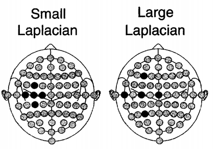
Size Variants

• Small Laplacian: Uses the 4 nearest neighbors (adjacent electrodes).
• Large Laplacian: Uses the next-nearest neighbors (4 electrodes beyond the adjacent ones).

Practical Recommendations

1. Use for Focal Activity: Ideal for detecting localized brain signals (e.g., ERP components, focal epileptic spikes).
2. Avoid for Generalized Activity: Not suitable for studying widespread brain states.
3. Handle Edge Electrodes Carefully: Use approximations (e.g., averaging 3 neighbors for T7) to mitigate edge effects.
4. Choose the Right Variant:

• Use planar Laplacian for simplicity.
• Use spherical or realistic head model Laplacian for higher accuracy in research settings.

How to Choose the Best EEG Reference

Localized Waveforms (e.g., focal epileptic spikes, ERP components)

• Best Choices: Laplacian or bipolar montages.
• Why? These methods enhance spatial resolution by emphasizing local activity and reducing the influence of distant signals.
• Alternatives: Weighted average > average > common reference.

Widespread Waveforms (e.g., generalized seizures, global brain states)

• Best Choice: Common reference (e.g., Cz, linked mastoids).
• Why? Common references capture global activity effectively without suppressing widespread signals.
• Alternatives: Average > weighted average > Laplacian or bipolar.

Analysis of Asymmetry (e.g., hemispheric differences)

• Best Choice: Common reference (e.g., Cz, linked mastoids).
• Why? Preserves lateralized differences and avoids artificial suppression of asymmetry.
• Alternatives: Average or bipolar > Laplacian.

Detecting Electrode Artifacts

• Best Choices: Common reference or bipolar.
• Why? These methods make it easier to identify noisy or poorly connected electrodes.
• Alternatives: Average > Laplacian.

Special Consideration for High-Density EEG (>100 Electrodes)

• Best Choice: Average reference (excluding electrodes near the signal of interest).
• Why? Reduces the risk of reference contamination and provides a stable baseline for high-density recordings.

Practical Tips

• Preprocessing: Always clean your data (e.g., remove bad channels) before applying any reference scheme.
• Edge Effects: For Laplacian references, handle edge electrodes carefully (e.g., approximate with fewer neighbors).
• Flexibility: If unsure, test multiple references and compare results to ensure robustness.

Referencing in NeuroAnalyzer

Referencing to common channel(s).

reference_ce(eeg, ch = "Cz")

If more than one channel is used as reference, the average of these channels is used:

reference_ce(eeg, ch = ["Fp1", "Fp2"])

Referencing to common average (CAR):

reference_avg(eeg,
              exclude_fpo = true,
              exclude_current = true)

Weighted average:

reference_avg(eeg,
              weighted = true)

Tip: exclude_fpo=true will exclude Fp1, Fp2 (due to eye blinks), O1, O2 (due to head movements) from CAR calculation.

Tip: exclude_current=true will exclude current channel from CAR calculation.

Referencing to ipsilateral auricular electrodes:

reference_a(eeg, type = :i)

Referencing to contralateral mastoid electrodes:

eeg_tmp = deepcopy(eeg)
# we don't have mastoid channels, so let's pretend
edit_channel!(eeg_tmp, ch = "A1", field = :label, value = "M1")
edit_channel!(eeg_tmp, ch = "A2", field = :label, value = "M2")
reference_m(eeg_tmp, type = :c)

Referencing using planar Laplacian:

eeg_lap = reference_plap(eeg,
                         nn = 4,
                         weighted = false)
plot_topo(eeg_lap,
          ch = "eeg",
          tpos = 12,
          title = "Laplacian (4)")

eeg_lap = reference_plap(eeg,
                         nn = 6,
                         weighted = true)
plot_topo(eeg_lap,
          ch = "eeg",
          tpos = 12,
          title = "Weighted Laplacian (6)")

Tip: Planar Laplacian referencing requires electrode locations.

Referencing using spherical Laplacian:

reference_slap(eeg,
               nn = 4,
               weighted = true)

Tip: Spherical Laplacian referencing requires electrode locations.

Custom referencing, e.g. bipolar longitudinal:

eeg_bipl = reference_custom(
    eeg,
    ref_list = [
        "Fz-Cz",
        "Cz-Pz",
        "Fp1-F7",
        "Fp1-F3",
        "F7-T3",
        "T3-T5",
        "T5-O1",
        "F3-C3",
        "C3-P3",
        "P3-O1",
        "Fp2-F8",
        "Fp2-F4",
        "F8-T4",
        "T4-T6",
        "T6-O2",
        "F4-C4",
        "C4-P4",
        "P4-O2",
    ],
    ref_name = "longitudinal-BIP",
)

Tip: ref_list must contain the list of channel pairs.

Examples of other custom montages:

Bipolar transverse:

ref_list = [
    "Fp2-Fp1",
    "F8-Fp2",
    "F8-F4",
    "F4-Fz",
    "Fz-F3",
    "F3-F7",
    "Fp1-F7",
    "T4-C4",
    "C4-Cz",
    "Cz-C3",
    "C3-T3",
    "T6-P4",
    "P4-Pz",
    "Pz-P3",
    "P3-T5",
    "O2-O1",
]
ref_name = "transverse-BIP"

Bipolar longitudinal with the middle line intact:

ref_list = [
    "Fz",
    "Cz",
    "Pz",
    "Fp1-F7",
    "Fp1-F3",
    "F7-T3",
    "T3-T5",
    "T5-O1",
    "F3-C3",
    "C3-P3",
    "P3-O1",
    "Fp2-F8",
    "Fp2-F4",
    "F8-T4",
    "T4-T6",
    "T6-O2",
    "F4-C4",
    "C4-P4",
    "P4-O2",
]
ref_name = "longitudinal-BIP"

Bipolar longitudinal:

ref_list = [
    "Fp-Fz",
    "Fz-Cz",
    "Cz-Pz",
    "Pz-O",
    "Fp1-F7",
    "Fp1-F3",
    "F7-T7",
    "T7-P7",
    "P7-O1",
    "F3-C3",
    "C3-P3",
    "P3-O1",
    "Fp1-F7",
    "Fp2-F4",
    "F8-T8",
    "T8-P8",
    "P8-O2",
    "F4-C4",
    "C4-P4",
    "P4-O2",
]
ref_name = "longitudinal-BIP"

Custom montages may be loaded from a file:

ref_l, ref_n = import_montage(joinpath(NeuroAnalyzer.PATH, "montages", "bip_long.mnt"));
eeg_custom = reference_custom(eeg, ref_list = ref_l, ref_name = ref_n);

Example montage files are located in the montages/ folder.

Tip: The structure of the montage file is:

• First line: name of the montage, e.g. longitudinal-BIP
• Next lines: channel pairs or individual channels, e.g. Fz-Cz or Fp1
• Each channel/channel pair must be in a separate line

Editing already exiting montage:

edit_montage("montages/bip_long.mnt")

Tip: This will open the .mnt file in the text editor.