Filtering

Initialize NeuroAnalyzer

using NeuroAnalyzer
using CairoMakie
CairoMakie.activate!(type = "png")
using Statistics
NeuroAnalyzer.progress_bar = false
NeuroAnalyzer.Random.seed!(42)

# NEURO object with one channel from a signal vector
# (used in the examples below)
function signal2obj(s::Vector{Float64}, fs::Int64)
    obj = create_object(; data_type = "eeg")
    obj.header.recording[:sampling_rate] = fs
    add_channel!(obj;
                 data = reshape(s, 1, :, 1),
                 label = "s",
                 type = "eeg",
                 unit = "μV")
    create_time!(obj; fs = fs)
    return obj
end
# Makie figure and axis settings matching NeuroAnalyzer plots
fig_size = (900, 450)
ax_style = (titlesize = 18,
            xlabelsize = 18,
            ylabelsize = 18,
            xticklabelsize = 12,
            yticklabelsize = 12,
            xticks = LinearTicks(10),
            xminorticksvisible = true,
            xminorticks = IntervalsBetween(10),
            xautolimitmargin = (0, 0),
            yautolimitmargin = (0.1, 0.1))

# raw (unfiltered) EEG recording
eeg = import_edf("files/eeg/eeg.edf")

A filter changes the frequency content of a signal: it attenuates some frequencies and passes others. In EEG/MEG processing, filters are used to:

remove slow drifts and DC offsets (high-pass filter),
remove high-frequency noise, e.g. muscle activity (low-pass filter),
remove power-line noise at 50 or 60 Hz (band-stop or notch filter),
isolate a frequency band, e.g. alpha (band-pass filter), for analyses of amplitude or phase.

Filters are linear and time-invariant (LTI): the filtered sum of signals equals the sum of the filtered signals, and the filter acts in the same way at every time point. A signal can therefore be thought of as a sum of sine waves (see Fourier transform): the filter scales the amplitude of each sine wave and shifts its phase, without creating new frequencies.

Filtering is never free: every filter distorts the signal in time. Choosing a filter is a trade-off between how cleanly it separates frequencies and how much it smears the signal in time.

Filter Types

Type	Passes	Typical use in EEG
low-pass (LP)	frequencies below the cutoff	remove muscle activity and high-frequency noise
high-pass (HP)	frequencies above the cutoff	remove DC offsets, slow drifts, sweating artifacts
band-pass (BP)	frequencies between two cutoffs	isolate a band (e.g. alpha 8-12 Hz) for amplitude/phase
band-stop (BS)	all except frequencies between two cutoffs	remove line noise (50/60 Hz)
notch	all except one narrow band	remove line noise

The ideal filters above (a rectangular “brick-wall” response) cannot be built: a real filter needs a transition band between the frequencies it passes and those it stops.

Describing a Filter

Frequency response (magnitude, gain): how much each frequency is attenuated, usually in decibels:

\[ \text{gain [dB]} = 20 \log_{10} \frac{A_{out}}{A_{in}} \]

Gain	Amplitude passed	Power passed
0 dB	100%	100%
−3 dB	70.7%	50%
−6 dB	50%	25%
−20 dB	10%	1%
−40 dB	1%	0.01%
−60 dB	0.1%	0.0001%

pass band: the frequencies that are passed (gain close to 0 dB); small variations are the pass-band ripple,
stop band: the frequencies that are attenuated; the minimum attenuation is the stop-band attenuation,
transition band: between them; its width (bw in NeuroAnalyzer) determines how steep the filter is (roll-off),
cutoff frequency: a reference point in the transition band, usually the frequency at which the gain is −3 dB (half power) or −6 dB (half amplitude); which one depends on the filter design (see below), so the cutoff alone does not describe a filter.

Impulse response: the output of the filter when the input is a single impulse (one sample of 1, all other samples 0). The impulse response describes the filter completely: filtering is the convolution of the signal with the impulse response, and the frequency response is the Fourier transform of the impulse response. A sharp frequency response (narrow transition band) requires a long impulse response, i.e. more smearing in time.

Phase response: how much each frequency is shifted in time. A filter whose phase shift is proportional to frequency (linear phase) delays all frequencies by the same time (the group delay) and keeps the shape of the signal; a non-linear phase delays different frequencies differently and distorts the waveform.

FIR and IIR Filters

Digital filters are of two kinds:

FIR (finite impulse response): the output is a weighted sum of the current and past input samples:

\[ y[n] = \sum_{k=0}^{N-1} b_k \, x[n-k] \]

The weights \(b_k\) (the filter kernel, taps or coefficients) are the impulse response, which has a finite length of \(N\) samples.

IIR (infinite impulse response): the output also depends on past output samples (feedback):

\[ y[n] = \sum_{k=0}^{N} b_k \, x[n-k] - \sum_{k=1}^{M} a_k \, y[n-k] \]

Because of the feedback, the impulse response decays but never reaches exactly zero.

	FIR	IIR
impulse response	finite (N samples)	infinite (decays)
stability	always stable	stable if well designed (poles inside the unit circle)
phase	linear (symmetric kernel): constant delay	non-linear: frequency-dependent delay
length for a steep filter	long (hundreds to thousands of taps)	short (order 2-10)
computation	slower	faster
design parameters	cutoff, transition band width (or number of taps)	cutoff, order
typical EEG use	band-pass for phase analyses, steep LP/HP	HP/LP for preprocessing, notch

Order: for an FIR filter, the number of taps \(N\) (in some texts \(N - 1\)); for an IIR filter, the number of poles (the highest delay of the feedback). A higher order gives a steeper roll-off, but for FIR filters also a longer impulse response, and for IIR filters a longer ringing and a higher risk of numerical problems.

Poles and zeros

The transfer function of a filter (its Z-transform, see Z-transform below) is a ratio of two polynomials:

\[ H(z) = \frac{b_0 + b_1 z^{-1} + \ldots + b_N z^{-N}}{1 + a_1 z^{-1} + \ldots + a_M z^{-M}} = k \frac{(z - z_1)(z - z_2) \cdots}{(z - p_1)(z - p_2) \cdots} \]

The roots of the numerator are the zeros (\(z_i\), frequencies that are suppressed), the roots of the denominator the poles (\(p_i\), frequencies that are amplified), \(k\) is the gain. An IIR filter is stable if all its poles lie inside the unit circle; an FIR filter has all its poles at \(z = 0\) and is always stable.

A Butterworth band-pass filter, 10-20 Hz, order 4:

flt = filter_create(fprototype = :butterworth,
                    ftype = :bp,
                    cutoff = (10, 20),
                    order = 4,
                    fs = 100)
println("poles: ", length(flt.p), ", zeros: ", length(flt.z),
        ", gain: ", round(flt.k; sigdigits = 3))
println("all poles inside the unit circle: ", all(abs.(flt.p) .< 1))

poles: 8, zeros: 8, gain: 0.00482
all poles inside the unit circle: true

plot_polezero(flt.p, flt.z)

FIR Filters

The Window Method

The ideal (rectangular) frequency response corresponds to an infinitely long impulse response (a sinc function). The window method cuts it to a finite length and multiplies it by a window (a taper), which smooths the truncation. The result is a filter with a transition band (whose width depends on the length of the kernel) and ripples in the pass and stop bands (whose size depends on the window).

The kernel of a low-pass FIR filter, 35 Hz, transition band 10 Hz, at 256 Hz:

flt = filter_create(fprototype = :fir,
                    ftype = :lp,
                    cutoff = 35,
                    bw = 10,
                    fs = 256)
println("taps: ", length(flt))
# time of each tap relative to the center of the kernel
t = ((1:length(flt)) .- (length(flt) + 1) / 2) ./ 256
lines(t, flt;
      color = :black,
      figure = (size = fig_size,),
      axis = (ax_style...,
              title = "FIR low-pass kernel",
              xlabel = "Time [s]",
              ylabel = "Coefficient"))

taps: 85

The kernel is symmetric, so the filter has a linear phase.

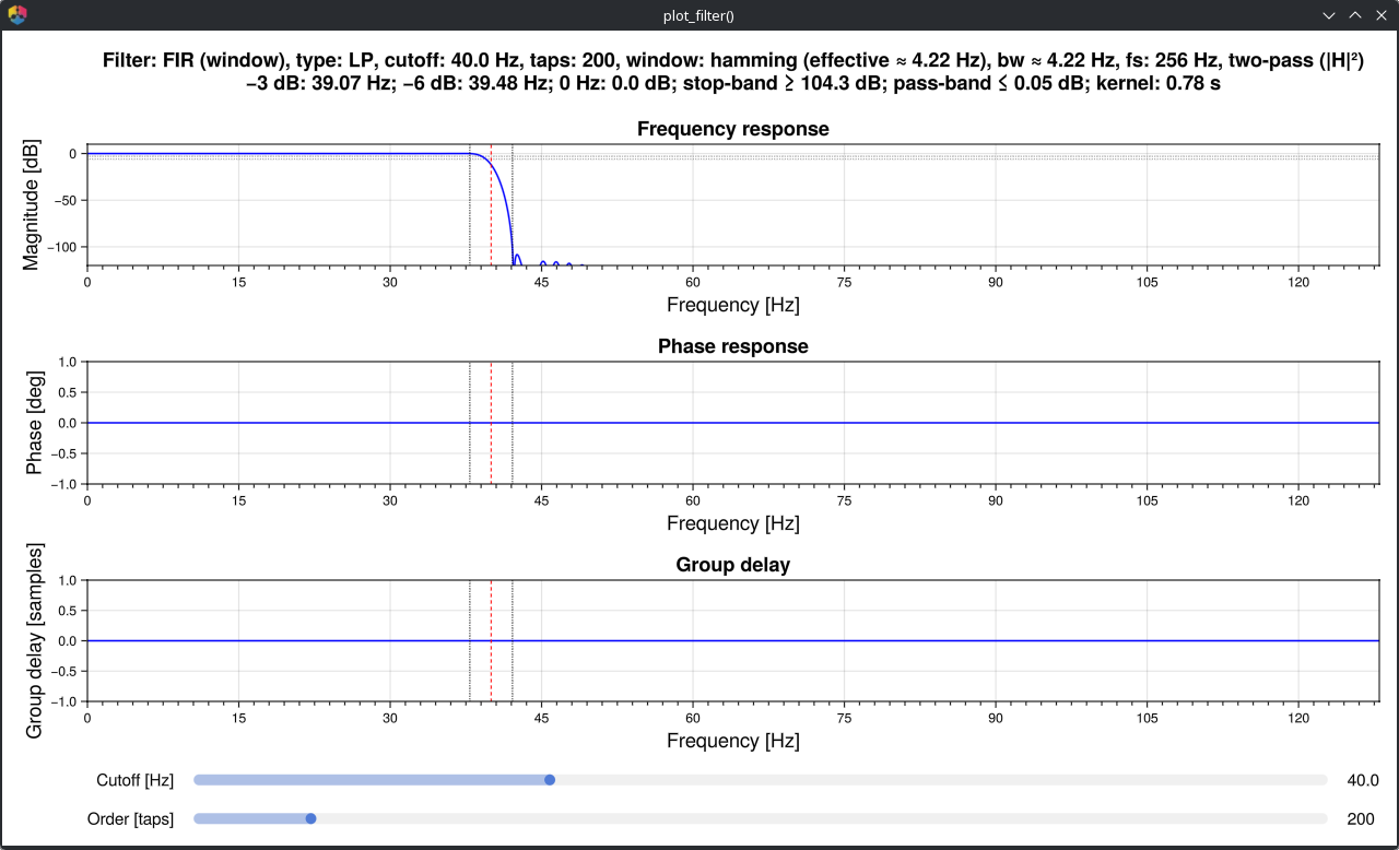
plot_filter() shows the frequency response, phase response and group delay of a filter designed with the same arguments as filter() (gui = false returns a static figure):

plot_filter(fs = 256,
            fprototype = :fir,
            ftype = :lp,
            cutoff = 35,
            bw = 10,
            gui = false)

The title lists the measured properties of the filter: −3 dB and −6 dB points, pass-band ripple, stop-band attenuation and the length of the kernel. For FIR filters designed with the window method, cutoff is the −6 dB point of a single pass (the middle of the transition band); with two passes (default) the gain at the cutoff is −12 dB, and the −3 dB point (32.8 Hz here) lies below the cutoff.

Windows

The window (window) sets the trade-off between the transition band width, the pass-band ripple and the stop-band attenuation. For the same transition band, windows with a higher attenuation need longer kernels:

println(rpad("window", 10), rpad("taps", 7), rpad("ripple [dB]", 14),
        "attenuation [dB]")
for w in [:rect, :hann, :hamming, :blackman]
    f = filter_create(fprototype = :fir,
                      ftype = :lp,
                      cutoff = 35,
                      bw = 10,
                      fs = 256,
                      window = w)
    r = filter_report(f;
                      fs = 256,
                      dir = :onepass,
                      ftype = :lp,
                      cutoff = 35,
                      bw = 10,
                      verbose = false)
    println(rpad(w, 10), rpad(length(f), 7), rpad(r.pass_dev, 14),
            r.stop_att)
end

window    taps   ripple [dB]   attenuation [dB]
rect      25     0.897         19.9
hann      81     0.056         43.9
hamming   85     0.025         49.5
blackman  141    0.002         72.8

The default Hamming window is a good compromise. A custom window (a vector of the length of the kernel) can be given with w; its length sets the number of taps.

Number of taps

When bw is given, the number of taps is computed from the transition band width; it can also be set directly with order. filter_order() returns the number of taps for a given transition band (rounded up to an odd number, which gives a linear-phase filter of any type):

\[ N = k \frac{f_s}{bw} \]

with \(k\) = 0.9 (rectangular), 3.1 (Hann), 3.3 (Hamming) or 5.5 (Blackman):

for bw in [10, 2, 0.5]
    n = filter_order(fprototype = :fir, fs = 256, bw = bw)
    println("bw = ", rpad(bw, 4), " Hz: ", rpad(n, 5), " taps (",
            round(n / 256; digits = 2), " s)")
end

bw = 10.0 Hz: 85    taps (0.33 s)
bw = 2.0  Hz: 423   taps (1.65 s)
bw = 0.5  Hz: 1691  taps (6.61 s)

A transition band of 0.5 Hz (e.g. for a high-pass filter at 0.5 Hz) requires a kernel of almost 7 s.

Other estimates of the number of taps:

fir_order_bw(): harris’ rule for a given stop-band attenuation \(A\) (dB): \(N = \frac{A}{22} \frac{f_s}{bw}\),
fir_order_f(): a rule of thumb for band-pass filters used in time-frequency analyses: the kernel should contain 4-5 cycles of the lowest frequency of interest.

println("harris (bw = 2 Hz, 60 dB): ", fir_order_bw(eeg; bw = 2, a = 60))
println("4-5 cycles of 8 Hz:         ", fir_order_f(eeg; f = 8))

harris (bw = 2 Hz, 60 dB): 349
4-5 cycles of 8 Hz:         (128, 160)

These are starting points; the response of the filter should always be checked with plot_filter() or filter_report().

Least-Squares and Remez Filters

Two other FIR designs optimize the kernel for a given transition band:

:firls: weighted least squares: minimizes the mean squared error between the actual and the ideal response; weights of the bands can be given with w,
:remez: Parks-McClellan (Remez exchange) algorithm: minimizes the maximum error (equiripple filter).

Both require bw; the number of taps is computed for a stop-band attenuation rs (default 53 dB) unless order is given:

plot_filter(fs = 256,
            fprototype = :remez,
            ftype = :bp,
            cutoff = (8, 12),
            bw = 2,
            gui = false)

IIR Filters

IIR filters are designed from analog prototypes, which differ in the shape of the frequency response:

Prototype	Pass band	Stop band	Roll-off	`cutoff` is
`:butterworth`	maximally flat	monotonic	slowest	the −3 dB point
`:chebyshev1`	ripple (`rp`)	monotonic	steeper	the end of the pass band (gain −`rp`)
`:chebyshev2`	flat	ripple (`rs`)	steeper	the start of the stop band (attenuation `rs`)
`:elliptic`	ripple (`rp`)	ripple (`rs`)	steepest	the end of the pass band (gain −`rp`)

rp is the pass-band ripple (default 0.5 dB) and rs the stop-band attenuation (default 20 dB). The four prototypes as low-pass filters, order 6, cutoff 35 Hz, one pass:

println(rpad("prototype", 14), "gain at 30 Hz   40 Hz      45 Hz")
for p in [:butterworth, :chebyshev1, :chebyshev2, :elliptic]
    f = filter_create(fprototype = p,
                      ftype = :lp,
                      cutoff = 35,
                      order = 6,
                      fs = 256)
    r = filter_report(f;
                      fs = 256,
                      dir = :onepass,
                      fcheck = [30, 40, 45],
                      verbose = false)
    println(rpad(p, 14), rpad(string(r.gain_at[30.0], " dB"), 15),
            rpad(string(r.gain_at[40.0], " dB"), 11),
            r.gain_at[45.0], " dB")
end

prototype     gain at 30 Hz   40 Hz      45 Hz
butterworth   -0.52 dB       -8.68 dB   -15.58 dB
chebyshev1    -0.465 dB      -14.716 dB -27.004 dB
chebyshev2    -1.088 dB      -20.05 dB  -30.117 dB
elliptic      -0.391 dB      -23.113 dB -20.199 dB

The Butterworth filter is the usual choice for EEG preprocessing: it has no ripple in the pass band, and its moderate roll-off produces less ringing than the steeper prototypes.

iir_order() estimates the order needed for a given transition band:

n = iir_order(eeg;
              fprototype = :butterworth,
              ftype = :lp,
              cutoff = 35,
              bw = 10)
println("Butterworth LP 35 Hz, transition band 10 Hz: order ", n)

Butterworth LP 35 Hz, transition band 10 Hz: order 11

A high-pass Butterworth filter, 0.5 Hz, order 4:

plot_filter(fs = 256,
            fprototype = :butterworth,
            ftype = :hp,
            cutoff = 0.5,
            order = 4,
            flim = (0, 5),
            gui = false)

Notch filter

:iirnotch is a second-order IIR filter that removes a narrow band around cutoff; bw is the width of the notch:

flt = filter_create(fprototype = :iirnotch, cutoff = 50, bw = 2, fs = 256)
r = filter_report(flt;
                  fs = 256,
                  fcheck = [45, 49, 50, 51, 55],
                  verbose = false)
for f in [45, 49, 50, 51, 55]
    println(f, " Hz: ", r.gain_at[Float64(f)], " dB")
end

45 Hz: -0.323 dB
49 Hz: -5.989 dB
50 Hz: -124.704 dB
51 Hz: -6.052 dB
55 Hz: -0.352 dB

Tip: Power-line noise often has harmonics (100, 150 Hz …) and varies in frequency and amplitude. A notch filter removes only one frequency; a low-pass filter below 50 Hz removes the line noise and its harmonics, and line noise removal methods remove it without filtering the neighboring frequencies.

Phase, Delay and Causality

A causal filter uses only the current and past samples: it can work in real time, but it delays the signal. A linear-phase FIR filter of \(N\) taps delays all frequencies by

\[ \tau = \frac{N - 1}{2 f_s} \]

e.g. 0.164 s for the 85-tap filter above. An IIR filter delays different frequencies by different times, which changes the shape of the signal.

A non-causal filter also uses future samples. Recorded signals are filtered offline, so non-causal filters can be used; the usual one is the two-pass (forward-backward, zero-phase) filter: the signal is filtered, reversed in time, filtered again and reversed back. The phase shifts of the two passes cancel, so the result has no delay and no phase distortion. The magnitude response is squared: the attenuation in dB is doubled, and the gain at the cutoff of a Butterworth filter is −6 dB instead of −3 dB.

The direction is set with dir:

:twopass (default): forward and backward (zero phase),
:onepass: forward only (causal, delayed),
:reverse: backward only (anti-causal).

A simulated ERP (P1 at 100 ms, N1 at 170 ms, P3 at 350 ms) filtered with a Butterworth low-pass filter at 10 Hz:

fs = 500
t = collect(-0.2:(1 / fs):0.8)
# Gaussian wave: latency t0 [s], amplitude a [μV], width w [s]
g(t0, a, w) = a .* exp.(-(t .- t0) .^ 2 ./ (2 * w^2))
erp = g(0.1, 3, 0.015) .+ g(0.17, -5, 0.02) .+ g(0.35, 8, 0.06)
# padded with 2 s of zeros on both sides (no edge artifacts)
pad = zeros(2 * fs)
obj = signal2obj(vcat(pad, erp, pad), fs)
idx = (length(pad) + 1):(length(pad) + length(erp))
erp_f = Dict{Symbol, Vector{Float64}}()
for d in [:onepass, :twopass]
    f = NeuroAnalyzer.filter(obj;
                             ch = "s",
                             fprototype = :butterworth,
                             ftype = :lp,
                             cutoff = 10,
                             order = 4,
                             dir = d)
    erp_f[d] = f.data[1, idx, 1]
end
fig = Figure(size = fig_size)
ax = Axis(fig[1, 1];
          ax_style...,
          title = "Butterworth LP 10 Hz",
          xlabel = "Time [s]",
          ylabel = "Amplitude [μV]")
lines!(ax, t, erp; color = :black, label = "original")
lines!(ax, t, erp_f[:onepass]; label = "one pass")
lines!(ax, t, erp_f[:twopass]; label = "two passes")
axislegend(ax)
fig

for d in [:onepass, :twopass]
    println(rpad(d, 9), ": P3 peak at ",
            round(Int, 1000 * t[argmax(erp_f[d])]), " ms")
end

onepass  : P3 peak at 394 ms
twopass  : P3 peak at 350 ms

The one-pass filter delays the P3 by about 40 ms and changes the shape of the components; the two-pass filter keeps the latencies.

Tip: Two-pass filters spread the signal backward in time as well as forward: a sharp event (e.g. a stimulus artifact or a response) can produce filter artifacts before it occurred. When the onset of an effect matters (e.g. ERP onset latencies), check the result with a causal filter.

Filter Artifacts

Distortion of the Signal

A filter changes every signal that has energy in its transition and stop bands, including the signal of interest. A high-pass filter removes slow drifts, but also slow ERP components such as the P3 or slow cortical potentials, and adds opposite-polarity deflections around them. The same simulated ERP, filtered with high-pass Butterworth filters (order 2, two passes):

fig = Figure(size = fig_size)
ax = Axis(fig[1, 1];
          ax_style...,
          title = "Butterworth HP, order 2",
          xlabel = "Time [s]",
          ylabel = "Amplitude [μV]")
lines!(ax, t, erp; color = :black, label = "original")
for c in [0.1, 1, 2]
    f = NeuroAnalyzer.filter(obj;
                             ch = "s",
                             fprototype = :butterworth,
                             ftype = :hp,
                             cutoff = c,
                             order = 2)
    s = f.data[1, idx, 1]
    lines!(ax, t, s; label = "HP $c Hz")
    println("HP ", rpad(c, 4), "Hz: P3 ",
            round(maximum(s[t .> 0.25]); digits = 1), " μV, N1 ",
            round(minimum(s[0.13 .< t .< 0.22]); digits = 1), " μV")
end
axislegend(ax)
fig

HP 0.1 Hz: P3 7.7 μV, N1 -5.2 μV
HP 1.0 Hz: P3 5.7 μV, N1 -6.3 μV
HP 2.0 Hz: P3 3.7 μV, N1 -5.5 μV

With a 0.1 Hz high-pass filter the ERP is almost unchanged; with 1-2 Hz the P3 is strongly reduced and the N1 becomes larger, an artificial effect created by the filter. For ERPs, high-pass filters above 0.1-0.3 Hz should be avoided.

Ringing: steep filters (narrow transition bands, high orders, elliptic and Chebyshev prototypes) respond to sharp transients (spikes, steps, artifacts) with oscillations at the cutoff frequency, which can be mistaken for brain oscillations.

Edge Artifacts

At the start and end of a signal the filter has no data before (or after) it: the kernel overlaps the missing samples and the output is distorted for about the length of the impulse response. Long kernels (low cutoffs, narrow transition bands) produce long edge artifacts; a high-pass filter at 0.5 Hz can distort several seconds.

Edge artifacts are avoided by filtering the continuous signal and splitting it into epochs afterwards. Filtering short epochs puts edges into every epoch:

e = crop(keep_channel(eeg; ch = "eeg"); seg = (100, 160))
# filter, then epoch
e1 = epoch(NeuroAnalyzer.filter(e;
                                ch = "all",
                                fprototype = :butterworth,
                                ftype = :hp,
                                cutoff = 0.5,
                                order = 4);
           ep_len = 2)
# epoch, then filter
e2 = NeuroAnalyzer.filter(epoch(e; ep_len = 2);
                          ch = "all",
                          fprototype = :butterworth,
                          ftype = :hp,
                          cutoff = 0.5,
                          order = 4)
d = abs.(e1.data .- e2.data)
println("mean |difference|, first 0.25 s of epochs: ",
        round(mean(d[:, 1:64, :]); digits = 1), " μV")
println("mean |difference|, 1.0-1.25 s of epochs:   ",
        round(mean(d[:, 257:320, :]); digits = 1), " μV")

mean |difference|, first 0.25 s of epochs: 189.5 μV
mean |difference|, 1.0-1.25 s of epochs:   32.5 μV

The epochs filtered separately differ from the correctly filtered signal everywhere (a 2-s epoch is shorter than the response of a 0.5 Hz filter), most at their edges. filter() warns when it is applied to an epoched object.

If a short segment must be filtered, pad it (e.g. with mirrored data) or taper its edges (multiply by a window such as Tukey) before filtering, and discard the edges afterwards.

Filtering EEG in Practice

Typical settings:

Filter	Setting	Notes
high-pass	0.1 Hz (ERPs), 0.5-1 Hz (other)	removes drifts; higher cutoffs distort slow components; 1 Hz is common before ICA
low-pass	30-45 Hz (ERPs, clinical), higher for gamma	removes muscle activity and line noise
notch	50 or 60 Hz	only if line noise remains and the band around it is not analyzed
band-pass	band of interest	for amplitude envelopes and phase (Hilbert transform); FIR, two passes

Guidelines:

filter as little as possible: every filter distorts the signal; analyses in the frequency domain (power spectra) often need no filtering at all,
filter the continuous signal, before epoching,
use two-pass (zero-phase) filters for offline analyses,
check the filter (plot_filter(), filter_report()) and the filtered signal,
report the filter in publications: type, prototype, cutoff and how it is defined (−3 dB or −6 dB), order or transition band, and direction (one or two passes).

The recording filtered 0.5-35 Hz (Butterworth high-pass, FIR low-pass):

eeg_f = NeuroAnalyzer.filter(eeg;
                             ch = "all",
                             fprototype = :butterworth,
                             ftype = :hp,
                             cutoff = 0.5,
                             order = 4)
NeuroAnalyzer.filter!(eeg_f;
                      ch = "all",
                      fprototype = :fir,
                      ftype = :lp,
                      cutoff = 35,
                      bw = 10)

The power spectra of the raw and filtered signals: the raw signal is dominated by the line noise at 50 Hz (and its harmonic at 100 Hz) and contains slow drifts; the filters remove both and keep the EEG activity between them:

s_raw = crop(eeg; seg = (100, 160))
s_flt = crop(eeg_f; seg = (100, 160))
p_raw = psd(s_raw; ch = "O1", db = true)
p_flt = psd(s_flt; ch = "O1", db = true)
fig = Figure(size = fig_size)
ax = Axis(fig[1, 1];
          ax_style...,
          title = "O1",
          xlabel = "Frequency [Hz]",
          ylabel = "Power [dB]")
lines!(ax, p_raw.f, vec(p_raw.p); label = "raw")
lines!(ax, p_flt.f, vec(p_flt.p); label = "0.5-35 Hz")
axislegend(ax)
fig

Filtering in NeuroAnalyzer

filter() designs and applies a filter in one step (filter!() modifies the object in place):

eeg_lp = NeuroAnalyzer.filter(eeg;
                              ch = "eeg",
                              fprototype = :fir,
                              ftype = :lp,
                              cutoff = 35,
                              bw = 10)

Argument	Meaning
`ch`	channels to filter
`fprototype`	`:fir`, `:firls`, `:remez`, `:butterworth`, `:chebyshev1`, `:chebyshev2`, `:elliptic`, `:iirnotch`
`ftype`	`:lp`, `:hp`, `:bp`, `:bs` (not used by `:iirnotch`)
`cutoff`	cutoff in Hz; a tuple `(f1, f2)` for `:bp` and `:bs`
`order`	number of taps (FIR) or order (IIR); computed from `bw` for FIR filters if not given
`bw`	transition band width in Hz (FIR, notch width for `:iirnotch`)
`window`, `w`	FIR window (`:rect`, `:hann`, `:hamming`, `:blackman`) or a custom window/weight vector
`rp`, `rs`	pass-band ripple and stop-band attenuation in dB (Chebyshev, elliptic)
`dir`	`:twopass` (default), `:onepass`, `:reverse`
`preview`	if `true`, plot the response of the filter without filtering

The measured properties of the filter are printed (unless verbose is off) and stored in the processing history:

println(last(eeg_lp.history))

filter_apply(obj; ch=[1, 2, 3, 4, 5, 6, 7, 8, 9, 10, 11, 12, 13, 14, 15, 16, 19, 20, 21], dir=:twopass) [FIR, taps=85, dir=:twopass; -3 dB at 32.805 Hz; -6 dB at 33.782 Hz; 0 Hz: 0.0 dB; pass-band dev ≤ 0.05 dB; stop-band att ≥ 97.4 dB]

Designing and applying a filter in two steps

filter_create() designs the filter (returns the FIR kernel or the IIR filter), filter_report() measures it, and filter_apply() applies it, e.g. to several objects:

flt = filter_create(fprototype = :butterworth,
                    ftype = :hp,
                    cutoff = 0.5,
                    order = 4,
                    fs = sr(eeg))
eeg_hp = filter_apply(eeg; ch = "eeg", flt = flt)

r = filter_report(flt; fs = sr(eeg), verbose = false)
println(r.summary)

IIR, order=4, dir=:twopass; -3 dB at 0.559 Hz; -6 dB at 0.5 Hz; 0 Hz: -12306.106 dB

Previewing a filter

# response of the filter, the signal is not filtered
NeuroAnalyzer.filter(eeg;
                     ch = "eeg",
                     fprototype = :fir,
                     ftype = :lp,
                     cutoff = 35,
                     bw = 10,
                     preview = true)
# interactive filter designer
plot_filter(eeg;
            fprototype = :fir,
            ftype = :lp,
            cutoff = 35,
            bw = 10)

Smoothing Filters

Smoothing filters are simple low-pass filters that work in the time domain. They are useful for removing noise from slowly changing signals (e.g. fNIRS, pupil size, behavioral data) and for removing spikes. A test signal (2 Hz sine wave with noise and three spikes):

fs = 256
t = collect(0:(1 / fs):(2 - 1 / fs))
s = 10 .* sin.(2π * 2 .* t) .+ 2 .* randn(length(t))
s[[100, 250, 400]] .+= [40, -30, 35]
obj = signal2obj(s, fs)
lines(t, s;
      color = :black,
      figure = (size = fig_size,),
      axis = (ax_style...,
              title = "Test signal",
              xlabel = "Time [s]",
              ylabel = "Amplitude [μV]"))

Filter	Function	Each sample is replaced by	Good for
moving average	`filter_mavg()`	the (weighted) mean of \(2k + 1\) samples around it	random noise
moving median	`filter_mmed()`	the median of \(2k + 1\) samples around it	spikes, outliers
Savitzky-Golay	`filter_sg()`	the value of a polynomial fitted to `window` samples around it	noise, keeping peak heights and widths
polynomial	`filter_poly()`	a polynomial fitted to consecutive windows	slow signals

s_mavg = filter_mavg(obj; ch = "s", k = 8).data[1, :, 1]
s_mmed = filter_mmed(obj; ch = "s", k = 8).data[1, :, 1]
s_sg = filter_sg(obj; ch = "s", order = 3, window = 31).data[1, :, 1]
fig = Figure(size = fig_size)
ax = Axis(fig[1, 1];
          ax_style...,
          title = "Smoothing filters",
          xlabel = "Time [s]",
          ylabel = "Amplitude [μV]")
lines!(ax, t, s; color = (:gray, 0.5), label = "signal")
lines!(ax, t, s_mavg; label = "moving average (k = 8)")
lines!(ax, t, s_mmed; label = "moving median (k = 8)")
lines!(ax, t, s_sg; label = "Savitzky-Golay (3, 31)")
axislegend(ax; position = :rb)
fig

The moving average smears the spikes over its window; the moving median removes them.

Moving average

The moving average of \(N = 2k + 1\) samples is an FIR filter with equal weights. Its frequency response has zeros at multiples of \(f_s / N\) and large side lobes, so it is a poor low-pass filter, but it is simple and does not create ringing. Its approximate cutoff (−3 dB) is

\[ f_c \approx \frac{0.443 f_s}{\sqrt{N^2 - 1}} \]

e.g. 6.7 Hz for \(k = 8\) at 256 Hz. A weighting window ww (length \(2k + 1\)) gives a weighted moving average, e.g. ww = [1, 2, 3, 2, 1] (with k = 2) a triangular one.

With a threshold t > 0, filter_mavg() and filter_mmed() replace only the samples outside mean ± t × SD of the signal, which removes outliers and keeps the rest of the signal unchanged:

s_out = filter_mmed(obj; ch = "s", k = 8, t = 3).data[1, :, 1]
println("samples changed: ", count(s_out .!= s))

samples changed: 3

Gaussian Filter

filter_g() extracts the amplitude envelope of a frequency band: the FFT of the signal is multiplied by a Gaussian centered at frequency f (width gw in Hz), keeping only the positive frequencies, and transformed back. The result is the analytic signal of the band (as with the Hilbert transform); filter_g() returns its absolute value, the envelope:

The test signal is a 10 Hz oscillation whose amplitude changes slowly (between 2 and 8 μV), with a 20 Hz sine wave of 3 μV:

fs = 256
t = collect(0:(1 / fs):(10 - 1 / fs))
amp = 5 .+ 3 .* sin.(2π * 0.2 .* t)
s = amp .* sin.(2π * 10 .* t) .+ 3 .* sin.(2π * 20 .* t)
obj = signal2obj(s, fs)
env = filter_g(obj; ch = "s", f = 10, gw = 4).data[1, :, 1]
fig = Figure(size = fig_size)
ax = Axis(fig[1, 1];
          ax_style...,
          title = "Gaussian filter at 10 Hz",
          xlabel = "Time [s]",
          ylabel = "Amplitude [μV]")
lines!(ax, t, s; color = (:gray, 0.5), label = "signal")
lines!(ax, t, amp; color = :black, linestyle = :dash,
       label = "true 10 Hz amplitude")
lines!(ax, t, env; color = :red, label = "envelope (filter_g)")
axislegend(ax; position = :rb)
fig

The Gaussian has no sharp edges, so the filter does not ring; its frequency resolution is set by gw: a narrow Gaussian separates close frequencies but follows fast amplitude changes less precisely. The same Gaussian kernels are used by the filter-Hilbert (:gh) time-frequency method.

Z-Transform

The Z-transform describes a discrete-time signal or system in the complex plane:

\[ X(z) = \sum_{n=-\infty}^{\infty} x[n] \, z^{-n}, \qquad z = r e^{i\omega} \]

On the unit circle (\(r = 1\), \(z = e^{i\omega}\)) it is the discrete-time Fourier transform: the angle \(\omega\) goes from 0 (0 Hz) to \(\pi\) (the Nyquist frequency). Inside and outside the circle, it also describes exponentially decaying and growing signals, which makes it the natural tool for IIR filters.

Filtering (convolution in time) becomes multiplication in the Z-domain:

\[ Y(z) = H(z) \, X(z) \]

where \(H(z)\), the Z-transform of the impulse response, is the transfer function of the filter. For FIR and IIR filters it is the ratio of polynomials shown in Poles and zeros. Evaluated on the unit circle, \(H(e^{i\omega})\) is the frequency response: the gain at a frequency is low near a zero and high near a pole, and a pole outside the unit circle makes the impulse response grow without bound (an unstable filter).