Initialize NeuroAnalyzer
using NeuroAnalyzer
eeg = load("files/eeg.hdf")using NeuroAnalyzer
eeg = load("files/eeg.hdf")Electrode Naming by Brain Region
Each electrode is labeled based on the brain lobe or area it records from:
Midline Electrodes (Z)
FpZ, Fz, Cz, Pz, OzLeft/Right Hemisphere Conventions
Special Electrode Locations
Right, Left, and Reference/Common.G1 and G2).
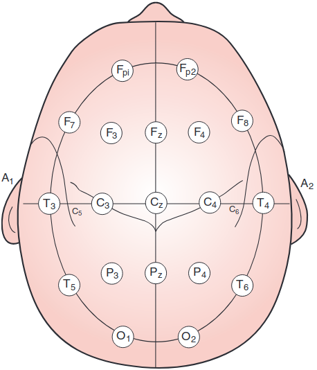
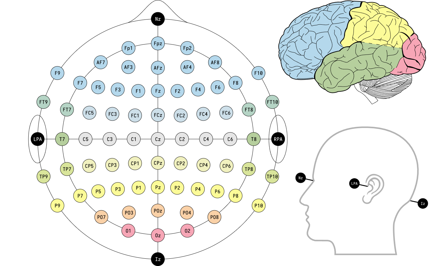
The Modified Combinatorial Nomenclature (MCM) extends the 10/20 system by adding intermediate electrode sites and updating naming conventions. It allows for higher spatial resolution in EEG recordings.
Electrode Naming and Placement
1, 3, 5, 7, 9 represent 10%, 20%, 30%, 40%, 50% of the inion-to-nasion distance, respectively.AF: Between Fp and FFC: Between F and CFT: Between F and TCP: Between C and PTP: Between T and PPO: Between P and ORenamed Electrodes
The MCN updates the following 10/20 system electrode names:
T3 → T7T4 → T8T5 → P7T6 → P810/5 System (5% System)
10/10 System (Chatrian, 1985)

or alternatively:
| Front to Back | Right to Left |
|---|---|
| nasion | tragus R |
| 10% | 10% |
| Fp | 8 |
| 20% | 20% |
| F | 4 |
| 20% | 20% |
| C | Z (midline) |
| 20% | 20% |
| P | 3 |
| 20% | 20% |
| O | 7 |
| 10% | 10% |
| inion | tragus L |
Electrode Naming and Placement
Types of Eye Movements Tracked

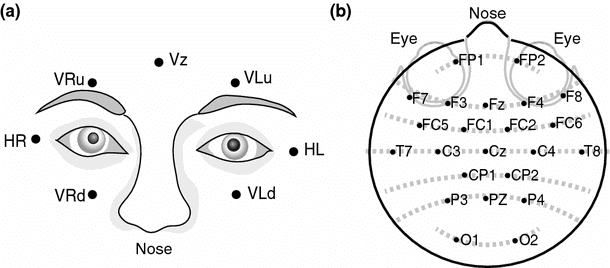
Purpose
Detecting and Removing Eye Movement Artifacts with ICA
Electrode Locations
ECG electrodes are placed at the following positions to record heart activity during EEG studies:
Purpose
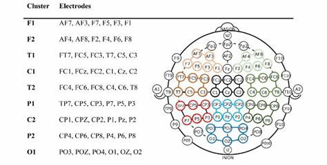
Overview
Electrode clusters refer to groups of electrodes that are analyzed together to study specific brain regions or functions. Clustering helps improve signal-to-noise ratio, spatial resolution, and functional interpretation of EEG data.
Common Electrode Clusters
Electrode clusters are often defined based on brain regions or functional networks:
| Cluster Name | Electrodes (10/20 System) | Brain Region/Function |
|---|---|---|
| Frontal | Fp1, Fp2, F3, F4, F7, F8, Fz | Frontal lobe: Executive function, attention, decision-making, and working memory. |
| Temporal | T7, T8, F7, F8, FT9, FT10 | Temporal lobe: Auditory processing, language, and memory. |
| Central | C3, C4, Cz, FC1, FC2, FC5, FC6 | Central region: Motor cortex, sensorimotor processing. |
| Parietal | P3, P4, P7, P8, Pz, CP1, CP2, CP5, CP6 | Parietal lobe: Spatial orientation, sensory integration, and attention. |
| Occipital | O1, O2, Oz, PO3, PO4, PO7, PO8 | Occipital lobe: Visual processing. |
| Midline | Fz, Cz, Pz, Oz | Midline structures: Default mode network, global brain states. |
| Fronto-Central | F3, F4, C3, C4, FC3, FC4 | Motor planning, cognitive control, and executive function. |
| Parieto-Occipital | P3, P4, O1, O2, PO3, PO4 | Visual-spatial integration and attention. |

Get channel names by channels picks:
# left fronto-temporal
channel_pick(eeg,
             pick=[:l, :f, :t])
5-element Vector{String}:
"Fp1"
"F3"
"F7"
"T3"
"T5"Tip: Available picks: :central (:c), :left (:l), :right (:r), :frontal (:f), :temporal (:t), :parietal (:p), :occipital (:o).
Get channel names by channels cluster:
channel_cluster(eeg,
                cluster=:f1)
3-element Vector{String}:
"Fp1"
"F3"
"F7"Tip: Available channel clusters are :f1, :f2, :t1, :t2, :c1, :c2, :p1, :p2, :o1.
Purpose of Electrode Clusters
Electrodes are positioned along X, Y and Z axes (Cartesian coordinates). The head center is at [0, 0, 0]. X axis is left-right, Y axis is back-front (the nose points towards +Y) and Z axis is bottom-top.

Electrode positions are stored in the OBJ.locs DataFrame. It contains the following columns:
labels: channel labelloc_theta: polar angleloc_radius: polar radiusloc_x: Cartesian Xloc_y: Cartesian Yloc_z: Cartesian Zloc_radius_sph: spherical radiusloc_theta_sph: spherical horizontal angleloc_phi_sph: spherical azimuth anglePolar coordinates are used to plot electrodes at XY-plane, while spherical coordinates are used to plot electrodes at XZ- and YZ-planes and in 3D view (internally converted to X, Y and Z coordinates). Alternatively, Cartesian coordinates are used for all projections.


Head dimensions are calculated on the basis of head circumference. Head is modeled as the perfect sphere with its center at the axes origin. Electrode positioning is based on 10-20 International system. In this system, electrode positions are based on the head and nasion-inion distance. Compared with the 10-20 standard, NeuroAnalyzer electrode positions are slightly tilted forward, making the horizontal plane at the Fpz/T7/Oz/T8 level perpendicular to the ground level and placing Cz channel at the head center.

Tip: For the horizontal view the fiducial points are inion (IN), nasion (NAS), left and right preauricular area (LPA, RPA)
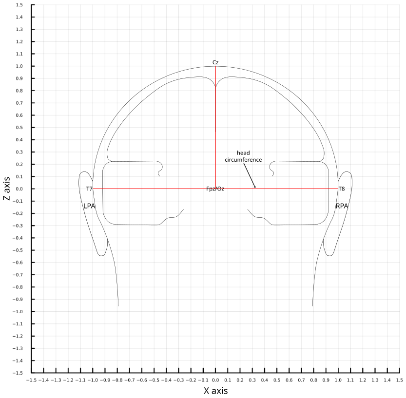
Tip: For the coronal view the fiducial points are left and right preauricular area (LPA, RPA).

Tip: For the sagittal view the fiducial points are inion (IN) and nasion (NAS).
Tip: In 19-channel systems, T7/T8 channels are sometimes labeled as T3/T4.
The position of fiducial EEG electrodes are:
The position of the fiducial head points are defined as:
NeuroAnalyzer.fiducial_points(nasion = (0.0, 1.03, -0.2), inion = (0.0, -1.03, -0.2), lpa = (-1.04, 0.2, -0.2), rpa = (1.04, 0.2, -0.2))Spherical Model Limitations
Visual Representations
Top View (XY-Plane):

Front View (YZ-Plane):

Side View (XZ-Plane):

NeuroAnalyzer Conventions for Imaging
Sagittal CT/MRI Images:
Practical Implications
CED
LOCS (Electrode Locations File)
chan_label, X, Y, Z (Cartesian coordinates), and optionally sph_theta, sph_phi, sph_radius (spherical coordinates).ELC (Electrode Location File)
Label, X, Y, Z coordinates, and sometimes Type (e.g., EEG, EOG).TSV (Tab-Separated Values)
label, x, y, z, and optionally additional metadata (e.g., theta, radius).SFP (Standardized Electrode Position File)
label, x, y, z (Cartesian coordinates), and optionally type (e.g., eeg, eog).CSD (Current Source Density)
label, x, y, z, and sometimes neighbors (for Laplacian calculations).GEO (Geometry File)
label, x, y, z, and optionally sphere_radius (for head model fitting).MAT (MATLAB Format)
.mat file storing electrode positions as a structure or table.labels, X, Y, Z, and optionally theta, phi, radius.import_locs() is a wrapper function that selects proper importing function based on file extension:
locs = import_locs("files/standard-10-20-cap19-elmiko.ced")| Row | label | loc_radius | loc_theta | loc_x | loc_y | loc_z | loc_radius_sph | loc_theta_sph | loc_phi_sph |
|---|---|---|---|---|---|---|---|---|---|
| String | Float64 | Float64 | Float64 | Float64 | Float64 | Float64 | Float64 | Float64 | |
| 1 | Fp1 | 1.0 | 108.0 | -0.31 | 0.95 | -0.03 | 1.0 | 108.02 | -1.72 |
| 2 | Fp2 | 1.0 | 72.0 | 0.31 | 0.95 | -0.03 | 1.0 | 71.98 | -1.72 |
| 3 | F7 | 1.0 | 144.0 | -0.81 | 0.59 | -0.03 | 1.0 | 144.04 | -1.72 |
| 4 | F3 | 0.65 | 129.0 | -0.55 | 0.67 | 0.5 | 1.0 | 129.0 | 30.0 |
| 5 | Fz | 0.51 | 90.0 | 0.0 | 0.72 | 0.7 | 1.0 | 90.0 | 43.82 |
| 6 | F4 | 0.65 | 51.0 | 0.55 | 0.67 | 0.5 | 1.0 | 51.0 | 30.0 |
| 7 | F8 | 1.0 | 36.0 | 0.81 | 0.59 | -0.03 | 1.0 | 35.96 | -1.72 |
| 8 | T3 | 1.0 | 180.0 | -1.0 | 0.0 | -0.03 | 1.0 | 180.0 | -1.72 |
| 9 | C3 | 0.51 | 180.0 | -0.72 | 0.0 | 0.7 | 1.0 | 180.0 | 43.82 |
| 10 | Cz | 0.0 | 0.0 | 0.0 | 0.0 | 1.0 | 1.0 | 0.0 | 90.0 |
| 11 | C4 | 0.51 | 0.0 | 0.72 | 0.0 | 0.7 | 1.0 | 0.0 | 43.82 |
| 12 | T4 | 1.0 | 0.0 | 1.0 | 0.0 | -0.03 | 1.0 | 0.0 | -1.72 |
| 13 | T5 | 1.0 | 216.0 | -0.81 | -0.59 | -0.03 | 1.0 | -144.04 | -1.72 |
| 14 | P3 | 0.65 | 231.0 | -0.55 | -0.67 | 0.5 | 1.0 | -129.0 | 30.0 |
| 15 | Pz | 0.51 | 270.0 | 0.0 | -0.72 | 0.7 | 1.0 | -90.0 | 43.82 |
| 16 | P4 | 0.65 | 309.0 | 0.55 | -0.67 | 0.5 | 1.0 | -51.0 | 30.0 |
| 17 | T6 | 1.0 | 324.0 | 0.81 | -0.59 | -0.03 | 1.0 | -35.96 | -1.72 |
| 18 | O1 | 1.0 | 252.0 | -0.31 | -0.95 | -0.03 | 1.0 | -108.02 | -1.72 |
| 19 | O2 | 1.0 | 288.0 | 0.31 | -0.95 | -0.03 | 1.0 | -71.98 | -1.72 |
Loading electrode positions in the CED format:
locs = import_locs_ced("files/standard-10-20-cap19-elmiko.ced")Adding electrode positions to the NEURO object:
add_locs!(eeg, locs=locs)Alternatively, loading electrode positions directly into existing NEURO object:
load_locs!(eeg, file_name="files/standard-10-20-cap19-elmiko.ced")Preview electrodes:
plot_locs(locs,
          ch=1:19,
          grid=true,
          gui=false)
Tip: Grid is useful for placing electrodes manually.
Tip: IN: inion, NAS: nasion, RPA: right pre-auricular. LPA: left pre-auricular.
To select channels, use sch argument:
plot_locs(locs,
          ch=1:19,
          sch=[1, 2],
          head_labels=false,
          ch_labels=true,
          gui=false)
Previewing electrodes loaded into NEURO object:
plot_locs(eeg,
          ch="eeg",
          gui=false)
By default, for 2D plots, electrodes are placed using polar coordinates (planar theta and radius):
plot_locs(eeg,
          ch="eeg",
          cart=false,
          gui=false)
To use Cartesian (X, Y, Z) coordinates:
plot_locs(eeg,
          ch="eeg",
          cart=true,
          gui=false)
To plot a XZ plane (front, coronal):
plot_locs(eeg,
          ch="eeg",
          plane=:xz,
          gui=false)
To plot a YZ plane (side, sagittal):
plot_locs(eeg,
          ch="eeg",
          plane=:yz,
          gui=false)
To plot a small plot (e.g. to use it with another channels plot), use ps=:m or ps=:s option:
plot_locs(eeg,
          ch="eeg",
          sch="eeg",
          ps=:m,
          gui=false)
Tip: Channel labels are not shown if ps=:m or ps=:s.
Tip: Channel colors are consistent across various plot types.
Tip: It is recommended to disable channel labels for legibility.
Side view:
plot_locs(eeg,
          ch="eeg",
          ch_labels=false,
          plane=:yz)
┌ Warning: Found `resolution` in the theme when creating a `Scene`. The `resolution` keyword for `Scene`s and `Figure`s has been deprecated. Use `Figure(; size = ...` or `Scene(; size = ...)` instead, which better reflects that this is a unitless size and not a pixel resolution. The key could also come from `set_theme!` calls or related theming functions. └ @ Makie ~/.julia/packages/Makie/kJl0u/src/scenes.jl:264

Tip: It is recommended to disable channel labels for legibility.
To add locations plot locs to another plot:
ch = ["Fp1", "Fp2", "F3", "F4"]
p = NeuroAnalyzer.plot(eeg,
                       ch="eeg",
                       seg=(20, 30),
                       type=:butterfly,
                       avg=false,
                       gui=false)
pl = plot_locs(eeg,
               ch=ch,
               sch=ch,
               ps=:s,
               gui=false)
pp = add_pl(p, pl)
plot_save(pp,
          file_name = "images/add_pl.png")
Viewing detailed electrode data:
locs_details(eeg,
             ch="Fp1")
Label: Fp1
Theta: 108.0 (polar)
Radius: 1.0 (polar)
X: -0.31 (spherical)
Y: 0.95 (spherical)
Z: -0.03 (spherical)
Radius: 1.0 (spherical)
Theta: 108.02 (spherical)
Phi: -1.72 (spherical)(label = "Fp1", theta_pl = 108.0, radius_pl = 1.0, x = -0.31, y = 0.95, z = -0.03, theta_sph = 108.02, radius_sph = 1.0, phi_sph = -1.72)Editing electrode position:
edit_locs!(eeg,
           ch="eeg",
           x=-1.0)
Converting spherical to Cartesian coordinates:
locs_sph2cart!(locs)Converting Cartesian to spherical coordinates:
locs_cart2sph!(locs)Converting Cartesian to spherical coordinates:
locs_cart2sph!(locs)Flipping axes (frontal channels should be at the top):
locs_flipx!(locs)
locs_flipy!(locs)

locs_flipy!(locs, planar=false)
locs_flipy!(locs, spherical=false)
locs_flipx!(locs, planar=false)
locs_flipx!(locs, spherical=false)

locs_flipz!(locs)

locs_swapxy!(locs)
Rotate=ing electrode locations:
# rotate around z axis
locs_rotz(locs, a=10)
# rotate around y axis
locs_roty(locs, a=10, cart=false)
# rotate around x axis
locs_rotx(locs, a=10, polar=false)
Tip: a specifies angle of rotation (in degrees). Positive angle rotates anti-clockwise.
Sometimes electrode locations may require scaling (polar radius value is being multiplied by the scaling factor):
locs_scale!(locs, r=1.2)Alternatively locations may be maximized to a unit circle:
locs_maximize!(locs)Save electrode positions (CED, LOCS and TSV format are supported), format will be selected based on the file name extension:
locs_export(eeg,
            file_name="files/standard-10-20-cap19-elmiko.locs")
locs_export(locs,
            file_name="files/standard-10-20-cap19-elmiko.ced")
locs_export(locs,
file_name="files/standard-10-20-cap19-elmiko.tsv")Previewing electrodes in 3-D:
p = plot_locs3d(eeg,
                ch="eeg",
                sch=["Fp1", "Fp2"],
                gui=false)
plot_save(p, file_name="images/plot_locs3d.png")
Tip: If gui parameter is true, the plot window is interactive; otherwise is just returns the rendered plot.
When interactive: you can rotate the view by left-clicking and dragging, span the view by right-clicking and dragging and zoom using the mouse wheel.
Keyboard shortcuts:
t: top viewr: right viewl: left viewf: front viewb: back viewHome: reset the views: save the view as PNG imageTip: By default, for 3D plots, electrodes are placed using Cartesian coordinates (x, y and z).
Drawing brain mesh together with electrode positions:
p = plot_locs3d(eeg,
            ch="eeg",
            sch=["Fp1", "Fp2"],
            mesh_type=:brain,
            gui=false)
plot_save(p, file_name="images/locs_brain.png")
p = plot_locs3d(eeg,
            ch="eeg",
            sch=["Fp1", "Fp2"],
            mesh_type=:head,
            gui=false)
plot_save(p, file_name="images/locs_head.png")
Tip: Mesh opacity can be set using mesh_alpha parameter, ranging from 1 (no opacity) to 0 (complete opacity).
Tip: The cam parameter sets initial camera position: first parameter is elevation, second - azimuth (both in degrees).
iedit(eeg)
For each channel, its label (e.g. “Fp1”), type (e.g. “eeg”) and units (e.g. “μV”) may be modified.
Also, electrode positions may be manually edit per each channel: polar radius and theta, Cartesian X, Y, Z and spherical radius, theta and phi coordinates may be entered in appropriate fields. Changes are automatically previewed in 4 views: top, front, side and 3D.
A set of transformations may be also applied to the whole locations set: flip over X/Y/Z axis, Swap X and Y axes, rotate around X/Y/Z axis, scale by a factor, normalize to a unit sphere. Each transformation is applied to selected set of coordinates (polar, Cartesian and spherical.)
Set of coordinates used for plotting is selected with the “Plot using Cartesian coordinates” switch: when off - polar coordinates are used for the top projection and spherical coordinates for the frontal, side and 3D projections; when on - Cartesian coordinates are used for all projections.
Also, coordinates may be transformed between projections (Cartesian → polar, Cartesian → spherical, polar → Cartesian, polar → spherical, spherical → Cartesian, spherical → polar).
All changes are done to a temporary object, use the “Apply” button to apply changes to the input object.
Tip: Since :eog and :ref channels are usually placed at fixed positions, they are not affected by transformations.