usingNeuroAnalyzerusingCairoMakieCairoMakie.activate!(type="png")# Quarto sets a default figure size (672 × 480 px), which overrides the sizes of# NeuroAnalyzer figures: remove itdelete!(CairoMakie.Makie.CURRENT_DEFAULT_THEME, :resolution)usingDataFramesusingStatisticsNeuroAnalyzer.progress_bar =false# Makie figure and axis settings matching NeuroAnalyzer plotsfig_size = (900, 450)ax_style = (titlesize =18, xlabelsize =18, ylabelsize =18, xticklabelsize =12, yticklabelsize =12, xticks =LinearTicks(10), xminorticksvisible =true, xminorticks =IntervalsBetween(10), xautolimitmargin = (0, 0), yautolimitmargin = (0.1, 0.1))# preprocessed recording (1000 s), EEG channels onlyeeg =load_neuro("files/eeg/eeg.hdf")eeg =keep_channel(eeg; ch ="eeg")# raw (unfiltered) recording of the same sessioneeg_raw =import_edf("files/eeg/eeg.edf")
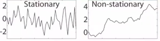
A signal is stationary when its statistical properties (mean, variance, frequency content, autocovariance) do not change over time. For example, for a group of signals recorded under the same conditions (an ensemble), the histograms of amplitudes are similar. A process is ergodic when a single recording is representative of the whole ensemble, i.e. averaging over time gives the same result as averaging over the ensemble.
A signal may be stationary in some properties only, e.g. it may have a constant mean (mean stationarity) but a changing variance (variance non-stationarity).
The EEG is quasi-stationary: it is stationary only over short segments (segments of several seconds, e.g. 10-second epochs, are usually treated as stationary). Its non-stationarity results from changes in the state of the neuronal assemblies during brain function (the state of the brain evolves over time), so non-stationarities are themselves informative about the underlying events.
Many signal processing methods (e.g. the Fourier transform, autoregressive models, many connectivity measures) assume stationarity. The EEG may be divided into segments to achieve local stationarity:
fixed segments (epochs)
adaptive segmentation, in which the boundaries are placed where the properties of the signal change
Stationarity can be used to choose the time windows of time-frequency analyses: it should be maintained for the length of the window used (the window of the short-time Fourier transform or the temporal width of the Gaussian taper of the Morlet wavelet).
Types of Stationarity
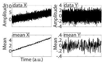
Mean stationarity: the signal is divided into non-overlapping windows and the mean of each window is calculated; the means of a stationary signal are similar.
X: mean non-stationarity
Y: mean stationarity
If a signal violates mean stationarity, the time-varying mean can be removed by:
detrending (or high-pass filtering),
computing the derivative,
calculating the time series of the time-varying mean and subtracting it from the signal.
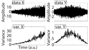
Variance stationarity: the variance of each window is calculated; the variances of a stationary signal are similar. Variance non-stationarity can be removed by normalizing (z-scoring) the signal within each window separately; this produces discontinuities at the window edges, which are detrimental to subsequent analyses unless they are performed separately in each window.
X: variance non-stationarity
Y: variance stationarity
Stationarity can also be assessed for higher-order moments, such as skewness (asymmetry of the distribution) or kurtosis (heaviness of its tails), or for any other statistical property of the signal (e.g. neg-entropy, or the Kullback-Leibler divergence between the amplitude distributions of the windows).
Phase stationarity: the unwrapped phase angle should increase monotonically and at a similar rate over time. Frequency is the first temporal derivative of the phase (instantaneous angular velocity), so phase stationarity and frequency stationarity are overlapping concepts: the derivative of the unwrapped phase (the instantaneous frequency) should be positive and similar over time. The phase is only meaningful for a narrow-band signal, so the signal should be band-pass filtered before assessing phase stationarity.
Covariance stationarity: the signal is divided into non-overlapping windows and the covariance matrix of the channels is calculated in each window; each matrix is compared with the matrix of the previous window. Covariance stationarity results in successive covariance matrices that are similar to each other, non-stationarity in dissimilar matrices.
The matrices may be compared using the Euclidean distance: corresponding elements of the two matrices are subtracted and squared, and all squared differences are summed (a sum of squared errors); the result is a time series of distances between successive matrices, which can be compared with the time-varying means and variances of the individual channels. Alternatively, the generalized eigenvalues of each two successive matrices can be calculated, and the distance taken as the ratio of the largest to the smallest eigenvalue.
Testing Stationarity
Statistical significance: the mutual information between the time series of the stationarity variable (mean, variance, etc.) and time quantifies how much information (entropy) they share. It detects both linear and non-linear, positive and negative relationships. Mutual information is the sum of the entropies of the two variables minus their joint entropy, where entropy is:
\[
H = -\sum p \times \log(p)
\]
where: \(p\) is the probability of observing a value in a particular bin (bins defined e.g. using the Freedman-Diaconis rule).
The mutual information is compared against its distribution expected by chance (no relationship between the stationarity variable and time), generated by randomly shuffling the time series and recomputing the mutual information.
Unit root tests: a unit root is related to the presence of significant autoregressive coefficients (current values can be predicted from the previous values in a way that makes the process drift); the most commonly used is the Augmented Dickey–Fuller (ADF) test.
Stationarity in NeuroAnalyzer
stationarity() calculates several measures of stationarity, selected by method:
method
Measure
Output shape
:mean
mean of each of window segments
(channels, window, epochs)
:var
variance of each of window segments
(channels, window, epochs)
:hilbert
derivative of the unwrapped Hilbert phase (radians per sample)
(channels, samples − 1, epochs)
:cov
Euclidean distance between the covariance matrices of adjacent segments of window samples
(segments − 1, epochs)
:adf
Augmented Dickey–Fuller statistic and p-value
(channels, 2, epochs)
Note that window is the number of segments for :mean and :var, but the segment length in samples for :cov.
Mean Stationarity
The raw recording contains a slow drift of the DC offset. Dividing the whole recording into 100 segments gives the mean of each segment:
The mean is not stationary: it decreases from about 900 μV to a few μV in Fp1 over the recording. After high-pass filtering (the preprocessed recording), the means are close to 0 μV throughout:
s_m =stationarity(eeg; ch = ["Fp1", "O1"], method =:mean, window =100)println("Fp1, range of means: ", round.(extrema(s_m[1, :, 1]); digits =2))
Fp1, range of means: (-0.25, 0.27)
Variance Stationarity
The variance of the preprocessed recording (1000 seconds) in 100 segments of 10 seconds:
The variance of O1 is increased in the first 300 seconds of the recording, both channels show short increases at about 110 and 305 seconds (the epochs with artifacts), and the variance of Fp1 slowly increases over the recording: the signal is not variance-stationary over its whole length, although it is approximately stationary within most 10-second segments.
Phase Stationarity
Phase stationarity is assessed for a narrow-band signal, here the alpha band (8–13 Hz) in 10-second epochs. The output (phase increment per sample, in radians) is converted to the instantaneous frequency in Hz by multiplying it by \(f_s / 2 \pi\):
eeg_alpha = NeuroAnalyzer.filter(eeg; ch ="eeg", fprototype =:butterworth, ftype =:bp, cutoff = (8, 13), order =4)e10_alpha =epoch(eeg_alpha; ep_len =10)s_p =stationarity(e10_alpha; ch ="O1", method =:hilbert)# instantaneous frequency in Hzfs =sr(eeg)f_inst = s_p[1, :, 1] .* fs ./ (2*pi)fig =Figure(size = fig_size)ax =Axis(fig[1, 1]; ax_style..., xlabel ="Time [s]", ylabel ="Frequency [Hz]", title ="Instantaneous frequency of alpha, O1, epoch 1")lines!(ax, e10_alpha.epoch_time[2:end], f_inst; color =:black)ylims!(ax, 0, 20)fig
The instantaneous frequency fluctuates around 10 Hz; short excursions (phase slips, including negative values outside the plotted range) occur where the amplitude of the alpha rhythm is low and its phase is poorly defined.
Covariance Stationarity
The distance between the covariance matrices of all EEG channels in adjacent 10-second (2560-sample) segments of the whole recording:
s_c =stationarity(eeg; ch ="eeg", method =:cov, window =10* fs)# time of the boundary between the compared segmentst_c = (1:size(s_c, 1)) .*10title ="Distance between covariance matrices"fig, ax, _ =scatterlines(t_c, s_c[:, 1]; color =:black, markersize =6, figure = (size = fig_size,), axis = (ax_style..., xlabel ="Time [s]", ylabel ="Distance", title = title))fig
Peaks indicate changes of the spatial structure of the signal between adjacent segments (e.g. transient artifacts or changes of the brain state).
Augmented Dickey–Fuller Test
The null hypothesis of the ADF test is that the signal has a unit root (it is non-stationary); p < 0.05 indicates a stationary signal. stationarity(; method = :adf) returns the ADF statistic and the p-value for each channel and epoch:
All channels are stationary in epoch 1. Very small p-values are reported as 0.0001. Note that the ADF test only detects a unit root (a random-walk-like drift); a signal with changing variance or frequency content may still be classified as stationary.